using RobustAndOptimalControl
using ControlSystems
using Plots
G = tf(200, [10, 1])*tf(1, [0.05, 1])^2; G = ss(G);
Gd = tf(100, [10, 1]); Gd = ss(Gd);
W1 = tf([1, 2], [1, 1e-6]); W1 = ss(W1);
K, γ, info = glover_mcfarlane(G, 1.1; W1);H∞ loop-shaping
The control design procedures introduced in the previous section were all based on models of uncertainty in the form of weighting filters and the corresponding \Delta blocks. Although we have provided some practical guidance on how to choose these weights, the modelling decisions can still be nontrivial. Shall we lump several parametric uncertainties into a single W\Delta term (perhaps assuming an input multiplicative uncertainty)? Or shall we dedicate a separate weighted \Delta term for each parametric uncertainty? Shall the model of the system assume uncertainty at each input? Shall output uncertainties also be included? Shall we include the uncertainty in the delay? And how about uncertainty in the order of the system? These are all questions that must be asked and answered. But how far shall we go with our quest for an accurate characterization of modelling inaccuracy (uncertainty)?
Coprime factor uncertainty
It turns out that there is yet another configuration of the \Delta blocks that is does not need specification of weighting filters and at the same time describes a fairly rich uncertainty family. This configuration is called coprime factor uncertainty. Do not let the mathematically sounding name scare you. It is actually very practical and useful. But some formal definitions are inevitable.
First, we assume the model of the system comes in the form of a fraction of two stable transfer functions as in G(s) = \frac{N(s)}{M(s)}, where N(\cdot) and M(\cdot) are such stable transfer functions; we write N(\cdot), M(\cdot)\in\mathcal{RH}_{\infty}, where \mathcal{RH}_{\infty} is a formal notation for the set of proper and stable rational transfer functions.
CautionTransfer function as a fraction of two polynomials vs a fraction of two stable transfer functions
Recall that the transfer function is a fraction of two polynomials. For example, G_0(s) = \frac{s+3}{s-1}. The same transfer function can also be expressed as a fraction of two stable transfer functions, for our example, G_0(s) = \frac{\frac{s+3}{s+p}}{\frac{s-1}{s+p}}, where p>0, and the two proper and stable transfer functions that define the ratio are N(s) = \frac{s+3}{s+p} and M(s) = \frac{s-1}{s+p}.
This whole concept can also be extended to MIMO systems. Recall that a convenient analogy of the concept of a transfer function as a fraction of two polynomials to MIMO systems is a fraction of two polynomial matrices. Now, instead of fractions of polynomial matrices, here we are going to consider fractions of stable matrix transfer functions. Since these are matrices, we need to distinguish between the left and right fractions. Here we show a left fraction: \mathbf G_0(s) = \mathbf M_\mathrm{L}^{-1}(s)\mathbf N_\mathrm{L}(s), where \mathbf M_\mathrm{L}(s) and \mathbf M_\mathrm{L}(s) are proper and stable matrix transfer function, which we write as \mathbf M_\mathrm{L}(s)\in\mathcal{RH}_{\infty}^{n\times n} and \mathbf N_\mathrm{L}(s)\in\mathcal{RH}_{\infty}^{n\times m}.
So far, co good. We have just reformatted the nominal model. Now we add the uncertainty. We do it in the following way. We consider two (stable) uncertainty blocks \Delta_\mathrm{N} and \Delta_\mathrm{M}. This time, however, we impose the bound slightly differently: \|[\Delta_\mathrm{N}\;\;\Delta_\mathrm{M}]\|_{\infty}\leq\epsilon, where \epsilon is a some positive number.
A (model of a) SISO uncertain system is then G(s) = \frac{N(s)+\Delta_\mathrm{N}(s)}{M(s)+\Delta_\mathrm{M}(s)}, and for a MIMO system we have \mathbf G(s) = (\mathbf M_\mathrm{L}(s)+\bm\Delta_\mathrm{M}(s))^{-1}(\mathbf N(s)+\bm\Delta_\mathrm{N}(s)). \tag{1}
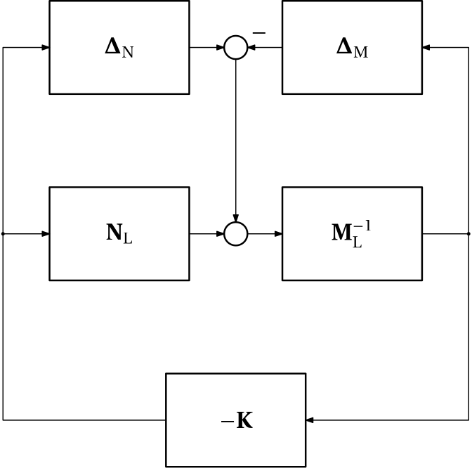
In words, both the numerator and denominator transfer functions are assumed to be additively perturbed by their own uncertainty blocks. The model in Eq. 1 is called a coprime factor uncertainty model, its block diagram interpretation is in Fig. 1.

We summarize the key peculiarities of this new uncertainty model compared to what we have covered before
- The two uncertainty blocks, \Delta_N and \Delta_M, are not normalized.
- The two uncertainty blocks \Delta_N and \Delta_M are only constrained by a single \mathcal H_\infty norm bound on the combined block [\Delta_N\;\;\Delta_M].
- There are no frequency-dependent weights.
Admittedly, this model is not intuitive. Indeed, it not possible to tell which of the two deltas is responsible for which source of uncertainty. However, it appears that we do not have to worry about this. However unintuitive, it does cover a broad family of uncertainties of various kinds.
And as the model contains no weighting filters, the only parameter of the model is thus the single positive number \epsilon that serves as an upper bound on [\Delta_N\;\;\Delta_M].
We now close a loop with a feedback controller \mathbf K around this uncertain system as in Fig. 2.
We redraw this in the format of our good old friend – an upper LFT of a nominal closed-loop system with respect to the uncertainty block as in Fig. 3.
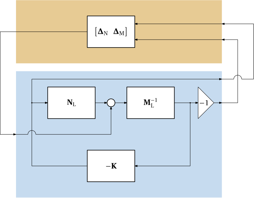
Let’s now determine the transfer function(s) of the one-input-two-output blue subsystem in Fig. 3.
\begin{bmatrix} -\mathbf K \mathbf{M}_\mathrm{L}^{-1} (\mathbf I+\mathbf{N}_\mathrm{L}\mathbf K \mathbf{M}_\mathrm{L}^{-1})^{-1}\\ -\mathbf{M}_\mathrm{L}^{-1} (\mathbf I+\mathbf{N}_\mathrm{L}\mathbf K \mathbf{M}_\mathrm{L}^{-1})^{-1} \end{bmatrix}
Since the delta blocks can have an arbitrary phase, we can ignore the minus sign in the above expression. In addition, we can also use the so-calle push-through identity.
NotePush-through identity
Consider two matrices \mathbf A and \mathbf B of compatible dimensions, \mathbf A invertible. Then \mathbf A(\mathbf I+\mathbf B\mathbf A)^{-1} = (\mathbf I + \mathbf A\mathbf B)^{-1}\mathbf A.
We get \begin{aligned} \begin{bmatrix} \mathbf K (\mathbf I+\mathbf{M}_\mathrm{L}^{-1} \mathbf{N}_\mathrm{L}\mathbf K )^{-1}\mathbf{M}_\mathrm{L}^{-1} \\ (\mathbf I+\mathbf{M}_\mathrm{L}^{-1} \mathbf{N}_\mathrm{L}\mathbf K )^{-1}\mathbf{M}_\mathrm{L}^{-1} \end{bmatrix} &= \begin{bmatrix} \mathbf K (\mathbf I+\mathbf{G}\mathbf K )^{-1}\mathbf{M}_\mathrm{L}^{-1} \\ (\mathbf I+\mathbf{G}\mathbf K )^{-1}\mathbf{M}_\mathrm{L}^{-1} \end{bmatrix}\\ &= \begin{bmatrix} \mathbf K \\ \mathbf I\end{bmatrix} (\mathbf I+\mathbf{G}\mathbf K )^{-1}\mathbf{M}_\mathrm{L}^{-1} \end{aligned}
Robust stability condition invoking the small gain theorem
We can now apply the small gain theorem to the LFT of the system we have just derived and the uncertainty block. The condition of robust stability is
\left\|\begin{bmatrix} \mathbf K \\ \mathbf I\end{bmatrix} (\mathbf I+\mathbf{G}\mathbf K )^{-1}\mathbf{M}_\mathrm{L}^{-1}\right\|_\infty < \frac{1}{\epsilon}.
CautionWhen previously introducing the small gain theorem, we assumed a normalized uncertainty
You may find the right-hand side of the above inequality puzzling. After all, we introduced the small gain theorem as \|\mathbf M\|_\infty<1. But recall that in that case we assumed that the uncertainty was normalized, that is, \|\bm \Delta\|_\infty \leq 1. Here, however, we did not enforce normalization and assumed that the uncertainty is bounded by \epsilon.
No \gamma iteration needed
For convenience, we label the achieved norm as \gamma \coloneqq \left\|\begin{bmatrix} \mathbf K \\ \mathbf I\end{bmatrix} (\mathbf I+\mathbf{G}\mathbf K )^{-1}\mathbf{M}_\mathrm{L}^{-1}\right\|_\infty.
We have learned previously, that when solving the \mathcal H_\infty optimal control problem, the existing methods only aim at finding a solution that achieves the bound on the norm. This bound is then iterated on – \gamma iteration. A pleasant property of the current problem is, that no \gamma iteration is needed – the optimal (the smallest) \gamma can be computed analytically:
\begin{aligned}
\gamma^\star &= (1-\|[\mathbf N_\mathrm{L}\;\mathbf M_\mathrm{L}]\|_{H}^{2})^{-\frac{1}{2}}\\
&= (1+\rho(\bm X\bm Z))^{\frac{1}{2}},
\end{aligned}
where H stands for Hankel norm (we do not need to go into the details right now), \bm Z\succ is the unique positive definite solution to the ARE
(\mathbf A-\mathbf B\mathbf S^{-1}\mathbf D^\top \mathbf C)\bm Z + \bm Z(\mathbf A-\mathbf B\mathbf S^{-1}\mathbf D^\top \mathbf C)^\top - \bm Z\mathbf C^\top \mathbf R^{-1}\mathbf C\bm Z + \mathbf B\mathbf S^{-1}\mathbf B^\top = \mathbf 0,
where
\mathbf R = \mathbf I+\mathbf D\mathbf D^\top,\quad \mathbf S = \mathbf I+\mathbf D^\top \mathbf D,
and \bm X\succ 0 uniquely solves the ARE
(\mathbf A-\mathbf B\mathbf S^{-1}\mathbf D^\top \mathbf C)^\top \bm X + \bm X(\mathbf A-\mathbf B\mathbf S^{-1}\mathbf D^\top \mathbf C) - \bm X\mathbf B\mathbf S^{-1}\mathbf B^{T}\bm X + \mathbf C^\top \mathbf R^{-1}\mathbf C = \mathbf 0.
The optimal (the smalles) \gamma then determines the largest \epsilon for which robust stability is guaranteed \epsilon_{\max} = \frac{1}{\gamma^\star}.
Robust stabilization by a central controller
Having computed the \gamma^\star, it turns out wise not to set \gamma to this smallest possible value but something a bit larger, say
\gamma = 1.1\gamma^\star, or so. We will see the reason a few lines below.
State-space realization of a controller that achieves
\left\|\begin{bmatrix} \mathbf K \\ \mathbf I\end{bmatrix} (\mathbf I+\mathbf{G}\mathbf K )^{-1}\mathbf{M}_\mathrm{L}^{-1}\right\|_\infty \leq \gamma.
can then be formed as (we remind that the equality sign is abused here in the common way)
\mathbf K = \left[
\begin{array}{l|l}
\mathbf A+\mathbf B\mathbf F+\gamma^2(\mathbf L^\top)^{-1}\mathbf Z\mathbf C^\top(\mathbf C+\mathbf D\mathbf F) & \gamma^2(\mathbf L^\top)^{-1}\mathbf Z\mathbf C^\top\\
\hline
\mathbf B^\top \bm X & -\mathbf D^\top
\end{array} \right]
where
\begin{aligned}
\mathbf F &= -\mathbf S^{-1}(\mathbf D^\top\mathbf C+\mathbf B^\top \bm X),\\
\mathbf L &= (1-\gamma^2)\mathbf I+\bm X\bm Z.
\end{aligned}
That \gamma should be set larger than \gamma^\star can be seen from the definition of \mathbf L – it avoids the singularity of \mathbf L.
ImportantDidactic point
We now want to emphasize an obvious didactic point. By stating all these equations, we do not mean to imply that their derivation “is obvious” or “is left as an exercise”, not to speak of “they must be memorized in order to be able to solve control problems”. Derivation of these results (and similarly for other parts of our \mathcal H_\infty andventure) is not trivial and we do not regard it as a part of our course. We can certainly have much value from these results just by using them. On the other hand, interested students can can certainly digest the details of the derivation provided in the literature – it is not much more complicated mathematics than the one used to develop the LQR theory, just a bit more work.
Glover-McFarlane \mathcal H_\infty loop-shaping procedure
Finally we show how the robust stabilization procedure can be used to design a controller that also achieve some desired performance of the closed-loop system. The procedure atributed consits of two steps:
- Design shaping filters that shape the magnitude frequency response of the open-loop transfer function of the nominal system.
- Robustly stabilize the shaped system against the coprime factorization uncertainty.
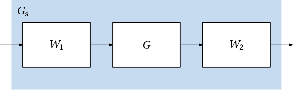
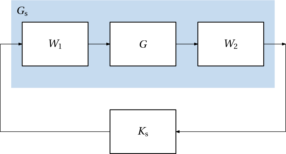
While designing the shaping filters, both input and output shaping filters can, in principle, be used for MIMO systems. The shaped plant is then given by \mathbf G_\mathrm{s}(s) = \mathbf W_\mathrm{2}(s)\mathbf G(s)\mathbf W_\mathrm{1}(s), see also Fig. 4.
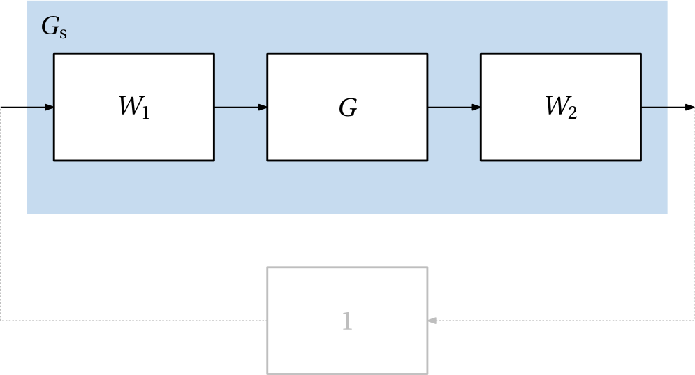
We can also view the design of shaping filters as a design of a nominal feedback controller whose only responsibility is to guarantee the desired performance. The series interconnection of the two shaping filters defines this controller, see Fig. 5 (note the absence of the minus sign). This viepoint is useful if we already have a controller that achieves the desired performance, but fails to guarantee robustness. For example, a nonrobust LQG or PID controller. But note that in principle, we do not even expect that the shaping filter guarantee a closed-loop stability. They should only focus on the shape of the magnitude frequency response, while they can freely ignore the phase, and consequently also the closed-loop stability.
A controller that robustly stabilizes this shaped plant against the coprime factor uncertainty is then designed using the Glover-McFarlane method, see Fig. 6 (note the absence of the minus sign – the minus must be a part of of the controller).
Once the controller robustly stabilizing the shaped plant is designed, we can then combine it with the shaping filters to form the final controller. When provisions for the unit gain of the closed-loop transfer function from the reference to the output is made, the resulting feedback interconnection looks like the one in
Example 1 (Loop-shaping design for SISO plant) This is Example 9.3 from [1]. The plant is a SISO system with the following transfer function G(s) = \frac{200}{10s+1} \frac{1}{(0.05s^2+1)^2}.
The disturbance model is G_\mathrm{d}(s) = \frac{100}{10s+1}.
The disturbance model gives us some guidance as for the desired closed-loop bandwidth. The closed-loop response of the plant output to the disturbance (in the current model we assume the disturbace added to the plantu output) is given by S(s)G_\mathrm{d}(s). We want to have the corresponding magnitude frequency response small at frequencies at which the disturbance is nonnegligible. Assuming the model is normalized (see [1, p. 4]), |S(j\omega)| should be small at the frequencies where G_\mathrm{d}(j\omega) \geq 1. In this case it is 10 rad/s. Within this bandwidth we want to have the best disturbance rejection possible.
The Bode plots of the plant and then both the nonrobust and the robustified open-loop transfer functions are at Fig. 8.
Show the code
bodeplot([G, info.Gs, G*K], lab=["G" "" "Initial GK" "" "Robustified GK" ""],lw=2)
The four important closed-loop transfer functions are at Fig. 9.
Show the code
Gcl = extended_gangoffour(G, K)
bodeplot(Gcl, lab=["S" "KS" "GS" "T"], plotphase=false,lw=2)
A time response of the closed-loop system with respect to a unit step disturbance for both the nominal nonrobust and the robustified controllers is at Fig. 10. Apparantly, the robustified controller achieve the same performance when it comes to the peak error and time constant, but the response is much less oscillatory, which reflects a more robust stability of the closed-loop system.
Show the code
plot(step(Gd*feedback(1, info.Gs), 3), lab="Initial controller",lw=2)
plot!(step(Gd*feedback(1, G*K), 3), lab="Robustified controller",lw=2)
References
[1]
S. Skogestad and I. Postlethwaite, Multivariable Feedback Control: Analysis and Design, 2nd ed. Wiley, 2005. Available: https://folk.ntnu.no/skoge/book/