using ControlSystems
G = tf(1, [2, 3])
W1 = tf(4, [5, 6])
W2 = tf(7, [8, 9])
W3 = tf(10, [11, 12])
P = [W1 -W1*G; 0 W2; 0 W3*G; 1 -G]
P = ss(P)
size(P.A,1)7Here we formulate the general problem of \mathcal{H}_\infty-optimal control. There are two motivations for this:
For the latter, recall that \|\mathbf G\|_{\infty} = \sup_{u\in\mathcal{L}_{2}\backslash \emptyset}\frac{\|\bm y\|_2}{\|\bm u\|_2}, in which we allow for vector input and output signals, hence MIMO systems.
Now, for particular control requirements, we build the generalized plant \mathbf P such that after closing the feedback loop with the controller \mathbf K as in Fig. 1,

these requirements are satisfied if the stabilizing controller minimizes the amplification of the exogenous inputs (disturbances, references, noises) into the regulated outputs. In other words, we want to make the regulated outputs as insensitive as possible to the exogenous inputs. When the sizes of the inputs and outputs are quantified using the \mathcal L_2 norm, what we have is the \mathcal{H}_\infty optimization problem \boxed {\operatorname*{minimize}_{\mathbf K \text{ stabilizing}}\|\mathcal{F}_{\mathrm l}(\mathbf P,\mathbf K)\|_{\infty}.}
Numerical solvers exist in various software environments. Before we at least comment on what is under the hood of these solvers, we first how the mixed-sensitivity problem can be formulated as a standard \mathcal{H}_\infty optimization problem. After all, this was one of the two motivations for this section.
We now show how the mixed-sensitivity problem discussed previously can be reformulated within as the standard \mathcal{H}_\infty optimization problem. We consider the full (containing all the three components) mixed-sensitivity problem. At first, we restrict ourselves to SISO plants, but this is purely for notational convenience as the extension to the MIMO case is seamless. The mixed-sensitivity problem is formulated as \operatorname*{minimize}_{K \text{ stabilizing}} \left\| \begin{bmatrix} W_1S\\W_2KS\\W_3T \end{bmatrix} \right\|_{\infty}, which obviously considers a closed-loop system with one input and three outputs. With only one exogenous input, we must choose its role. Say, the only exogenous input is the reference signal. The closed-loop system for which the norm is minimized is in the following block diagram Fig. 2.
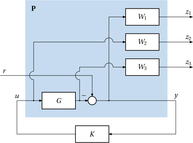
The matrix transfer function for generalized plant \mathbf P has two inputs and four outputs and it can then be written as \mathbf P = \left[\begin{array}{c|c} W_1 & -W_1G\\ 0 & W_2\\ 0 & W_3G\\ \hline 1 & -G \end{array}\right]. \tag{1}
A state space realization of this plant \mathbf P is then used as the input argument to the solver for the \mathcal{H}_\infty optimization problem. But note we must also tell the solver how the inputs and outputs are structured (the information provided by the internal horizontal and vertical lines in Eq. 1). In this case, the solver must be given the information that out of the two inputs, only the second one can be used by the controller, and out of the four outputs, only the fourth one is measured.
By the way, how would the block diagram and the generalized plant \mathbf P change if the output disturbance d was the only exogenous input instead? Hint: the change is minor.
The mixed-sensitivity problem only considers a single exogenous input (albeit a vector one). As a consequence, we cannot formulate the problem of simultaneous reference tracking and disturbance rejection within the mixed-sensitivity framework.
But now that we have seen that the mixed-sensitivity problem is reformulated/reformatted as the general \mathcal{H}_\infty optimal control problem, nothing prevents us from adding more inputs, outputs and whatever internal blocks to the generalized plants \mathbf P. Numerical solvers for the \mathcal{H}_\infty optimal control problem can also accept other types of generalized plants than those that correspond to the mixed-sensitivity problem.
For example, consider not only the reference input r but also the disturbance d_\mathrm{i} acting at the input to the plant G. This we can’t really express as a mixed-sensitivity problem. But we can express it as a standard \mathcal{H}_\infty optimal control problem. The block diagram is shown in Fig. 3.
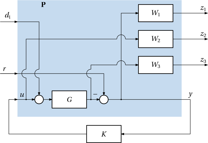
The generalized plant \mathbf P is now \mathbf P = \left[\begin{array}{cc|c} -W_1G & W_1 & -W_1G\\ 0 & 0 & W_2\\ W_3G & 0 & W_3G\\ \hline -G & 1 & -G \end{array}\right].
No surprise, the first column is equal to the third column as the input disturbance d_\mathrm{i} enters the plant in the same way as the control input u.
What if the measurement noise (corrupting additively the measured output y) needs to be added to the model? How would the block diagram and consequently the generalized plant \mathbf P change?
When forming the generalized plant \mathbf P using a software tool of our choice, we typically get a realization that is not minimal. For example, if the plant G and all the three weighting filters are first-order systems, the state-space model of the generalized plant \mathbf P in Eq. 1 obtained just by stacking the individual transfer functions horizontally and vertically into a matrix, is a seventh-order system (there are seven first-order systems in the generalized plant). However, if we take into consideration that out of the seven transfer function, only four are distinct, we can suspect that the generalized plant \mathbf P can be realized as a state-space model of a lower order.
using ControlSystems
G = tf(1, [2, 3])
W1 = tf(4, [5, 6])
W2 = tf(7, [8, 9])
W3 = tf(10, [11, 12])
P = [W1 -W1*G; 0 W2; 0 W3*G; 1 -G]
P = ss(P)
size(P.A,1)7Pmin = minreal(P, atol=1e-13, rtol=1e-13)
size(Pmin.A,1)4In our course have have no ambitions to derive the solution to the optimal control at the same level of detail as we did for the LQR problem. Here we only state the results.
The important difference between the \mathcal H_\infty optimal control problem and the LQR, LQG, and \mathcal H_2 optimal control problems is that for the former we have no closed-form formula for the optimal controller. We can only find a (stabilizing) controller that guarantees that the \mathcal{H}_\infty norm of the closed-loop system is less than a given threshold \gamma:
\operatorname*{find}_{\mathbf K \text{ stabilizing}}\|\mathcal{F}_{\mathrm l}(\mathbf P,\mathbf K)\|_{\infty} \leq \gamma.
For solving this problem of \mathcal H_\infty suboptimal control, several approaches exist. Here we only discuss the one known as Doyle–Glover-Khargonekar-Francis (DGKF) method, which based on solving two Riccati equations. This is frequently the default method in available solvers.
For a given LTI system modelled by the quadruple of matrices (\mathbf A, \mathbf B, \mathbf C, \mathbf D), and for a given \gamma > 0, search for positive definite \bm{X}\succ 0 and \bm{Y}\succ 0 solving two Riccati equations \begin{aligned} \mathbf{A}^\top \bm{X} + \bm{X}\mathbf{A} + \mathbf{C}_1^\top \mathbf{C}_1 + \bm{X}(\gamma^{-2}\mathbf{B}_1\mathbf{B}_1^\top -\mathbf{B}_2\mathbf{B}_2^\top )\bm{X} &= \mathbf 0,\\ \mathbf{A}\bm{Y} + \bm{Y}\mathbf{A}^\top + \mathbf{B}_1\mathbf{B}_1^\top + \bm{Y}(\gamma^{-2}\mathbf{C}_1^\top \mathbf{C}_1-\mathbf{C}_2^\top \mathbf{C}_2)\bm{Y} &= \mathbf 0, \end{aligned} such that \begin{aligned} \text{Re}\;\lambda_i(\mathbf{A}+(\gamma^{-2}\mathbf{B}_1\mathbf{B}_1^\top -\mathbf{B}_2\mathbf{B}_2^\top )\bm{X})&<0, \;\forall i,\\ \text{Re}\;\lambda_i(\mathbf A+\bm{Y}(\gamma^{-2}\mathbf{C}_1^\top \mathbf{C}_1-\mathbf{C}_2^\top \mathbf{C}_2)) &<0 ,\;\forall i, \end{aligned} and \rho(\bm{X}\bm{Y})<\gamma^2.
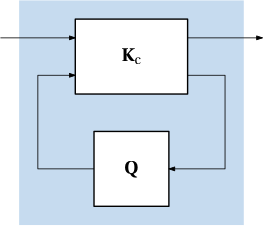
All stabilizing controllers that guarantee that the norm is <\gamma are given by the lower linear fractional transformation \mathbf K=\mathcal F_\mathrm{l}(\mathbf K_\mathrm{c},\bm Q), where \mathbf K_\mathrm{c} is given by \begin{aligned} \mathbf K_\mathrm{c}(s) &= \left[ \begin{array}{l|ll} \mathbf A + \gamma^{-2}\mathbf{B}_1\mathbf{B}_1^\top \bm{X}+\mathbf{B}_2\mathbf{F}+\mathbf{Z}\mathbf{L}\mathbf{C}_2 & -\mathbf{Z}\mathbf{L} & \mathbf{Z}\mathbf{B}_2\\ \hline \mathbf{F} & \mathbf{0} & \mathbf{I}\\ -\mathbf{C}_2 & \mathbf{I} & \mathbf{0} \end{array} \right]\\ \mathbf{F} &= -\mathbf{B}_2^\top \bm{X},\\ \mathbf{L} &=-\bm{Y}\mathbf{C}_2^\top,\\ \mathbf{Z} &= (\mathbf{I} -\gamma^{-2}\bm{Y}\bm{X})^{-1}, \end{aligned} and \mathbf Q(s) is an arbitrary stable transfer function satisfying \|\mathbf Q\|_{\infty}<\gamma.
This Q-parameterization of a controller in the form of a lower LFT is visualized in Fig. 4.
For \mathbf Q=\bm 0, we get the central controller \mathbf K(s) = \mathbf K_{\mathrm{c}_{11}}(s) = -\mathbf{Z}\mathbf{L}\left(s\mathbf{I}-(\mathbf A + \gamma^{-2}\mathbf{B}_1\mathbf{B}_1^\top \bm{X}+\mathbf{B}_2\mathbf{F}+\mathbf{Z}\mathbf{L}\mathbf{C}_2)\right)^{-1}\mathbf{F}.
It is useful to note that the order of the central regulator is that same as that of the generalized plant \mathbf P.
Consider the state-space model of the generalized plant parameterized by the quadruple of matrices (\mathbf A, \mathbf B, \mathbf C, \mathbf D), which can be partitioned as \left[ \begin{array}{l|ll} \mathbf A_{1} & \mathbf B_1 & \mathbf B_2\\ \hline \mathbf C_1 & \mathbf D_{11} & \mathbf D_{12}\\ \mathbf C_2 & \mathbf D_{21} & \mathbf D_{22} \end{array} \right].
Sufficient conditions for existence of \bm K minimizing \|F_l(P,K)\|_{\infty} are:
In some literature, the assumption that \mathbf D_{11}=0 and \mathbf D_{22}=0 is made. But it is not necessary. It only simplifies the formulas. If the original problem does not satisfy these assumptions, the original problem can be transformed.
Note that these are all just sufficient conditions. They rule out some degenerate cases. Even in those cases, the optimal solution may still exist.
We are now well aware that the LQG/\mathcal H_2 optimal controller can be separated into an observer and a state feedback controller. This fundamental property is beyond useful from both theoretical and practical points of view.
Can we get anything like that for the \mathcal H_\infty optimal controller? It turns out that this is the closest we can get: the central controller can be separated into an observer \dot{\hat{\bm x}} = \mathbf A\hat{\bm x} + \mathbf B_1\underbrace{\gamma^{-2}\mathbf B_1^\top \bm X\hat{\bm x}}_{\hat{\bm w}_{\text{worst}}} + \mathbf B_2\bm u + \mathbf Z\mathbf L(\mathbf C_2\hat{\bm x}-\bm y), and a state feedback \bm u=\mathbf F\hat{\bm x}.
Compared to a Kalman filter, here we have the extra term \mathbf B_1\hat{\bm w}_{\text{worst}}, where \hat{\bm w}_{\text{worst}} can be interpreted as an estimate of the worst-case disturbance. Consequently, this separation into an observer and a state feedback controller is of very limited use, which is unfortunate.
We will see later, however, that there is one particular setting (the robust \mathcal H_\infty loop-shaping), in which the \mathcal H_\infty optimal controller can be separated into an observer and a state feedback controller in the LQG sense.