For a given system, there may be some inherent limitations of achievable performance. However hard we try to design/tune a feedback controller, certain closed-loop performance indicators such as bandwidth, steady-state accuracy, or resonant peaks may have inherent limitations. We are going to explore these. The motivation is that once we know what is achievable, we do not have to waste time by chasing the unachievable.
At first it may look confusing that we are only formulating this problem of learning the limitations towards the end of our course. After all, one view of the optimal control theory is that is that it provides a systematic methodology for learning what is possible to achieve. Shall we need to know the shortest possible time in which the quadrotor can fly from one position and orientation to another, we just formulate the minimum-time optimal control problem and solve it. Even if at the end of the day we intend to use a different controller – perhaps one supplied commercially with a fixed structure like a PID controller – at least we can assess the suboptimality of such controller by comparing its performance with the optimal one.
ImportantOptimal control theory may help reveal the limitations
Indeed, this is certainly a fair and practical motivation for studying even those parts of optimal control theory that do not provide very practical controllers, such as the \mu synthesis returning controllers of rather high order even for low-order plants.
But we have also seen that the optimal control theory can also be used as a convenient tool to achieve certain performance requirements. For example, should we have some requirements on the closed-loop bandwidth and the attenuation of disturbances at low frequencies, the \mathcal H_\infty optimal control methods can be used to search for a controller that shapes the closed-loop transfer functions accordingly. It is then useful to be able to tell if the requirements are achievable or not.
In this section we are going to restrict ourselves to SISO systems. Then in the next section we will extend the results to MIMO systems.
Fundamental trade-off
The first limitation is captured by the following relation between the sensitivity function S(s) and the complementary sensitivity function T(s)\boxed{
S+T = 1.}
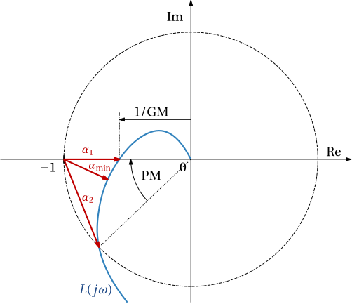
Magnitude and phase margins vs. sensitivity function
Using the generic Nyquist plot in Fig. 1, we define the smallest distance of the Nyquist plot to the critical point -1 as \alpha_{\min}. We can show that it is equal to the reciprocal value of the peak of the magnitude of the sensitivity function S(s), that is,
\alpha_{\min}=\inf_{\omega}\left|-1-K(j\omega)G(j\omega)\right|=\frac{1}{\|S(s)\|_{\infty}}.
Figure 1: Three different notions of distance of the Nyquist plot from the critical point -1: two are related to GM and PM, the third one is related to the peak in the magnitude of S
We can relate the gain margin (GM) and phase margin (PM) to other two distances \alpha_1 and \alpha_2 sketched in Fig. 1:
\mathrm{GM}=\frac{1}{1-\alpha_1}, \qquad \mathrm{PM}=2\arcsin\frac{\alpha_2}{2},
and as these distances lower-bounded by \alpha_{\min}, we get the following useful inequalities
\mathrm{GM}\geq\frac{M_S}{M_S-1},\qquad \mathrm{PM}\geq 2\arcsin\frac{1}{2M_S},
where M_S \coloneqq \|S\|_\infty. For commonly required values GM=2 a PM=30^\circ, we get M_S=2, which corresponds to 6 dB.
Clarification of the definition of bandwidth
The definition of the bandwidth that is often promoted in circuit and filter theory uses the complementary sensitivity function T(s), and it defined as the frequency \omega_\mathrm{B} up to which the magnitude |T(j\omega)| of the complementary sensitivity function is \approx 1 (typically the value of 1/\sqrt{2} is used). The motivation for this definition might be that the system can track references with the frequency content up to this frequency.
We state here another definition of bandwidth that is more appropriate for control systems – the frequency \omega_\mathrm{B} up to which the magnitude |S(j\omega)| of the sensitivity function is smaller than \approx 1 (again, typically the value of 1/\sqrt{2} is used). The motivation for this definition is that the system can reject disturbances with the frequency content up to this frequency.
While mostly the two definitions give similar values of the bandwidth, they can be quite different in some cases, as illustrated with the following example.
Example 1 (Two definitions of bandwidth) We consider the following open-loop transfer function
L(s) = \frac{-s + 0.1}{s(s+2.1)}.
The magnitude and phase frequency responses for the sensitivity and complementary sensitivity functions are in Fig. 2.
Figure 2: Bode plot of the sensitivity and complementary sensitivity functions
When determined from the magnitude frequency response |T(j\omega)|, the bandwidth is \approx 1 rad/s. But note that at this frequency the phase is already lagging by \approx 200 degrees. This means that even if the frequency content of the reference is not attenuated, the reference will be distorted so much that we can hardly claim that the system is still tracking it.
In contrast, the bandwidth determined from the magnitude frequency response |S(j\omega)| is well below 0.1 rad/s (it is \approx 0.036 rad/s). This means that the system can reject disturbances with the frequency content up to this frequency. And the phase is completely irrelevant here.
The step response of the system in Fig. 3 supports this preference for the latter definition. The bandwidth determined from the complementary sensitivity function would suggest that the time constant recognizable in the step response is \approx 1 second, while we can observe a time constant \approx 30 s, which is in much better agreement with 1/0.036.
Figure 3: Step response of the closed-loop system that demonstrates the difference between the two definitions of bandwidth
Interpolation conditions of internal stability
Consider that the plant modelled by the transfer function G(s) has a zero in the right half-plane (RHP), that is,
G(z) = 0, \; z\in \text{RHP}.
It can be shown that the closed-loop transfer functions S(s) and t(s) satisfy the interpolation conditions \boxed{
S(z)=1,\;\;\;T(z)=0
}
Proof. Showing this is straightforward and insightful: since no unstable pole-zero cancellation is allowed if internal stability is to be guaranteed, the open-loop transfer function L=KG must inherit the RHP zero of G, that is,
L(z) = K(z)G(z) = 0, \; z\in \text{RHP}.
But then the sensitivity function S=1/(1+L) must satisfy
S(z) = \frac{1}{1+L(z)} = 1.
Consequently, the complementary sensitivity function T=1-S must satisfy the interpolation condition T(z)=0.
Similarly, assuming that the plant transfer function G(s) has a pole in the RHP, that is,
G(p) = \infty, \; p\in \text{RHP},
which can also be formulated in a cleaner way (avoiding the infinity in the definition) as
\frac{1}{G(p)} = 0, \; p\in \text{RHP},
the closed-loop transfer functions S(s) and T(s) satisfy the interpolation conditions \boxed
{T(p) = 1,\;\;\;S(p) = 0.}
The interpolation conditions that we have just derived constitute the basis on which we are going to derive the limitations of achievable closed-loop magnitude frequency responses. But we need one more technical results before we can proceed. Most probably you have already encountered it in some course on complex analysis - maximum modulus principle. We state this result in the jargon of control theory.
Theorem 1 (Maximum modulus principle) For a function F(\cdot) of a complex variable s that is analytic in the closed right half-plane (RHP), it holds that
\sup_{\omega}|F(j\omega)|\geq |F(s_0)|\;\;\; \forall s_0\in \text{RHP}.
This can also be expressed compactly as
\|F(s)\|_\infty \geq |F(s_0)|\;\;\; \forall s_0\in \text{RHP}.
When restricted to rational (transfer) functions, the requirement of analyticity in the closer RHP is equivalent to the requirement that the transfer function has no poles in the RHP. In the control systems lingo these are stable transfer functions.
Now instead of some general stable transfer function F(s) we consider the weighted sensitivity function W_\mathrm{p}(s)S(s). And we restrict our attention to one particular complex number s in the RHP, namely, a RHP zero z of the plant transfer function G(s), that is, G(z)=0, \; z\in\mathbb C, \; \Re(z)\geq 0. Then the maximum modulus principle together with the interpolation condition S(z)=1 implies that
\|W_\mathrm{p}S\|_{\infty}\geq |W_\mathrm{p}(z)|.
Similar result holds for the weighted complementary sensitivity function W(s)T(s) and an unstable pole p of the plant transfer function G(s), when combining the maximum modulus principle with the interpolation condition T(p)=1
\|WT\|_{\infty}\geq |W(p)|.
These two simple results can be further generalized to the situations in which the plant transfer function G(s) has multiple zeros and poles in the RHP. Namely, if G(s) has N_p unstable poles p_i and N_z unstable zeros z_j,
As a special case, consider the no-weight cases W_\mathrm{p}(s)=1 and W(s)=1 with just a single unstable pole and zero. Then the limitations on the achievable closed-loop magnitude frequency responses can be formulated as
\|S\|_{\infty} > c, \;\; \|T\|_{\infty} > c, \;\;\;c=\frac{|z+p|}{|z-p|}.
Example 2 For G(s) = \frac{s-4}{(s-1)(0.1s+1)}, the limitations are
\|S\|_{\infty}>1.67, \quad \|T\|_{\infty}>1.67.
Limitations of the achievable bandwidth due to RHP zeros
There are now two requirements on the weighted sensitivity function that must be reconciled. First, the performance requirements
|S(j\omega)|<\frac{1}{|W_\mathrm{p}(j\omega)|}\;\;\forall\omega\;\;\;\Longleftrightarrow \|W_\mathrm{p}S\|_{\infty}<1
and second, the just derived consequence of the interpolation condition
\|W_\mathrm{p}S\|_{\infty}\geq |W_\mathrm{p}(z)|.
The only way to satisfy both is to guarantee that
|W_\mathrm{p}(z)|<1.
Now, consider the popular first-order weight
W_\mathrm{p}(z)=\frac{s/M+\omega_\mathrm{B}}{s+\omega_\mathrm{B} A}.
For one real zero in the RHP, the inequality |W_\mathrm{p}(z)|<1 can be written as
\omega_\mathrm{B}(1-A) < z\left(1-\frac{1}{M}\right).
Setting A=0 a M=2, the upper bound on the bandwidth follows
\boxed
{\omega_\mathrm{B}<0.5z.}
For complex conjugate pair
\omega_\mathrm{B}=|z|\sqrt{1-\frac{1}{M^2}},
and M=2, it follows that \omega_\mathrm{B}<0.86|z|.
Limitation on the achievable bandwidth due to unstable poles
Using the robust stability condition
|T(j\omega)|<\frac{1}{|W(j\omega)|}\;\;\;\forall\omega\;\;\;\Longleftrightarrow \|WT\|_{\infty}<1
and the interpolation condition
\|WT\|_{\infty}\geq |W(p)|,
it follows that the only way to satisfy both is to guarantee that
|W(p)|<1.
With the weight
W(s)= \frac{s}{\omega_\mathrm{BT}}+\frac{1}{M_\mathrm{T}}
we get a lower bound on the bandwidth
\omega_\mathrm{BT} > p\frac{M_\mathrm{T}}{M_\mathrm{T}-1},
from which it follows that for M_\mathrm{T}=2, \boxed
{\omega_\mathrm{BT}>2p.}
For complex conjugate pair:
\omega_\mathrm{BT}>1.15|p|.
Limitations due to time delay
Consider the problem of designing a feedback controller for reference tracking. An ideal closed-loop transfer function T(s) from the reference to the output satisfies T(s)=1. If the plant has a time delay, the best achievable closed-loop transfer function T(s) is given by
T(s) = e^{-\theta s},
that is, the reference is perfectly tracked, albeit with some delay. The best achievable sensitivity function S(s) is then given by
S(s) = 1-e^{-\theta s}.
We now approximate the sensitivity function by the first-order Taylor expansion
S(s) \approx \theta s,
from which we can see that the magnitude frequency response of the sensitivity function is approximated by a linear function of frequency. Unit gain is achieved at about
\omega_{c}=1/\theta.
From this approximation, we can see that the crossover frequency, hence the bandwidth of the system is limited by the time delay \theta as
\boxed{
\omega_c < \frac{1}{\theta}.
}
Scaling of the model
Before we move on, we need to introduce the important concept of scaling. We consider the input-output model of the plant whose output is additively disturbed by the disturbance. Abusing the notation a bit (by using the same symbols for time-domain signals as well as their Laplace transform), we write the model as
\hat y(s) = \hat G(s)\hat u(s)+\hat G_\mathrm{d}(s) \hat d(t),\qquad \hat e(s) = \hat r(s)-\hat y(s).
We now collect the lower and upper bounds on the amplitude of the control input \hat u(t), estimates of the lower and upper bounds on the disturbance \hat d(t), and possibly the reference \hat r(t), and we also determine the lower and upper bounds on the amplitude of the regulation error \hat e(t), which guarantee satisfactory performance of the system. Once we have them, we can modify (scale) the original model so that it assumes that for the new (scaled) model, the amplitudes of all the variables are bounded by 1. The fact that after scaling all the above mentioned variables are bounded by 1, is also reflected in the notation as we remove the hats from the symbols, as in Fig. 4. Note that scaling with respect to the reference will generally call for introduction of a scaling gain R in the model of the plant.
Figure 4: Model of a plant with a disturbance model and a reference. The block R represents a scaling gain that is generally needed for scaling.
The procedure for modifying the original model is straigthforward, and since it is described on some two or three pages in the freely available part of [1, p. 5], we skip the details here.
From now on, we assume that the model of the plant and the disturbace is scaled.
Limitations due presence of disturbance
Disturbances also impose some limitations on the achievable performance. But we have to simplify a bit (actually quite a lot) here. In particular, we assume that the disturbance is a harmonic (sinusoidal) signal, or close to it. Since we also assume that the model is scaled, we write the disturbance as
d(t)=\sin(\omega t).
It is only for this class of inputs that the transfer function model predicts easily the amplitude of the output. In absence of control, and if r=0, the regulation error due to the disturbance d(t) is a harmonic signal too, that is,
e(t)=e_0\sin(\omega t+\phi),
where e_0 is the gain and \phi is the phase shift. Since we assume that the model is scaled, the amplitude e_0 of the regulation error must be bounded by one and hence
|G_\mathrm{d}(j\omega)|<1.
If this is not satisfied, we need a feedback. Since then the regulation error is given by
e(s)=S(s)G_\mathrm{d}(s)d(s),
we can express the requirement of an acceptably small regulation error as
|S(j\omega)G_\mathrm{d}(j\omega)|<1\; \forall \omega \quad \Longleftrightarrow \quad |S(j\omega)|<\frac{1}{G_\mathrm{d}(j\omega)}\; \forall \omega \quad \Longleftrightarrow \quad \|SG_\mathrm{d}\|_{\infty}<1.
Example 3 (Disturbance enforcing an upper bound on the sensitivity function) For the disturbance model
G_\mathrm{d}(s)=\frac{10}{100s+1},
the upper bound on the magnitude frequency response of the sensitivity function is in Fig. 5. This also enforces that the bandwidth of the system is at least 0.1 rad/s.
Figure 5: Magnitude frequency response of the (reciprocal) of the disturbance model
In words, the system must be able to attenuate the disturbances at the frequency range where the disturbance is strong enough (magnitude higher than one for a normalized model). We formally state the result as \boxed{
\omega_\mathrm{B}>\omega_\mathrm{d},
}
where \omega_\mathrm{d} is frequency where |G_\mathrm{d}(j\omega)|=1.
We can get additional limitation if the system has an RHP zero. Invoking the interpolation conditions of internal stability, we get the constraint
|G_\mathrm{d}(z)|<1.
Limitations due to saturation of actuators
We assume the standard input-output model including the disturbance model
y(s) = G(s)u(s)+G_\mathrm{d}(s)d(t),\qquad e(s) = r(s)-y(s),
and we assume that the model has already been scaled, that is, the control input is constrained by
|u(t)|<1.
We now refer to the ideal control
u(s)=G^{-1}(s)r(s)-G^{-1}(s)G_\mathrm{d}(s)d(s).
If we now assume that the disturbance is a harmonic signal (or close to it), the ideal control input is then also harmonic. And relying on the fact that the model has already been scaled so that a unit-amplitude disturbance can be assumed, the condition to avoid saturation is
|G^{-1}(j\omega)G_\mathrm{d}(j\omega)|<1\;\;\;\forall \omega,
which we can rewrite as \boxed{
|G(j\omega)|>|G_\mathrm{d}(j\omega)|\quad \forall \omega.}
In words, the gain of the plant must be larger than the gain of the disturbance model. We cannot overemphasize that scaling is crucial here.
Example 4 (Avoiding saturation of control inputs due to disturbance can conflict with the necessity to attenuate disturbances) We consider a stable plant transfer functions G(s) and the disturbance model G_\mathrm{d}(s) as in the code below.
In Fig. 6 we can see the magnitude frequency responses of a stable plant and a disturbance model. The condition that control is not saturated is satisfied up to the frequency below 1 rad/s (\approx 0.38 rad). But the disturbance model has the magnitude larger than 1 up to the frequency slightly above 10 rad/s (\approx 15 rad/s). This means that within the frequency range [0.38, 15] rad/s, saturation may occur. The danger of saturation is present at higher frequencies, but taking into consideration that the magnitude of the disturbance model is smaller than 1, there is no need to design the controller such that the bandwidth extends above 15 rad/s.
Figure 6: Magnitude frequency response of the plant and disturbance model
Example 5 (Avoiding saturation of control inputs due to disturbance can conflict with the necessity to stabilize the system) We consider an unstable plant transfer functions G(s) and the disturbance model G_\mathrm{d}(s) as in the code below.
In Fig. 7 we can then see their magnitude frequency responses. If it weren’t for the unstable pole in the plant transfer function, we could even decide not to design the controller at all, as the magnitude of the disturbance model is smaller than 1, which for a scaled model implies that no control is needed. But we do have to design a feedback controller in order to stabilize the system in the first place. The unstable pole at s=1 then imposes a constraint the bandwidth – it must be at least 2 rad/s. Hélas, the disturbance model is stronger at the frequency range [0.62, 2], which means that the control input may saturate.
S. Skogestad and I. Postlethwaite, Multivariable Feedback Control: Analysis and Design, 2nd ed. Wiley, 2005. Available: https://folk.ntnu.no/skoge/book/