Through this chapter we are stepping into the domain of robust control. We need to define a few keywords first.
Definition 1 (Uncertainty) Deviation of the mathematical model of the system from the real (mechanical, electrical, chemical, biological, …) system.
Definition 2 (Robustness) Insensitivity of specified properties of the system to the uncertainty.
While these two terms are used in many other fields, here we are tailoring them to the discipline of control systems, in particular their model-based design.
Definition 3 (Robust control) Not a single type of a control but rather a class of control design methods that aim to ensure robustness of the resulting control system. By convention, a robust controller is a fixed controller, typically designed for a nominal model. This is in contrast with an adaptive controller that adjusts itself in real time to the actual system.
Origins of uncertainty in models?
Physical parameters are not known exactly (say, they are known to be within ±10% or ±3σ interval around the nominal value).
Even if the physical parameters are initially known with a high accuracy, they can evolve in time, unmeasured.
There may be variations among the individual products of the same kind.
If a nonlinear system is planned to be operated around a given operating point, it can be linearized at that operating point, which gives a nominal linear model. If the system is then operated at a significantly different operating point, the corresponding linear model differs from the nominal one.
Our understanding of the underlying physics (or chemistry or biology or …) is imperfect, hence our model is imperfect too. In fact, our understanding can even be incorrect, in which case the model contains some discrepancies too. The imperfections of the model are typically observed at higher frequencies, while at low frequencies or at least at the model of the steady-state response the accuracy is typically better (referring to the frequency-domain modeling such as transfer functions).
Even if we are able to eventually capture full dynamics of the system in a model, we may opt not to do so. We may want to keep the model simple, even if less accurate, because time invested into modelling is not for free, of course.
Even if we can get a high-fidelity model with a reasonable effort, we may still prefer using a simpler (and less accurate) model for a controller design. The reason is that very often the complexity of the model used for model-based control design is reflected by the complexity of the controller; and high-complexity controllers are not particularly appreciated in industry.
Models of uncertainty (uncertainty in models)
There are several approaches to modelling (characterizing) of the uncertainty. They all aim – in one way or another – to expressing that instead of only a single (nominal) system, a whole family of systems needs to be considered. Depending on the mathematical frameworks used for characterization of such a family, there are two major classes of approaches.
Worst-case models of uncertainty
Probabilistic models of uncertainty
The former assumes sets of systems with no additional information about the structure of such sets. The latter imposes some probability structure on the set of systems – in other words, although in principle any member of the set possible, some may be more probable than the others. In this course we are focusing on the former, which is also the mainstream in the robust control literature, but note that the latter we already encountered while considering control for systems exposed to random disturbances, namely the LQG control. A possible viewpoint is that the random disturbance represents the uncertainty in the system.
Another classification of models of uncertainty is according to the actual aspect of the (model of the) system that is uncertain. We distinguish these two
Parametric uncertainty
Frequency-dependent (aka dynamical) uncertainty
Unstructured uncertainty
Structured uncertainty
Parametric uncertainty
This is obviously straightforward to state: some real (physical) parameters are uncertain. The conceptually simplest way to characterize such uncertain parameters is by considering intervals instead of just single (nominal) values.
Example 1 (A pendulum on a cart) Within the state equation
\dot{\bm x}(t) =
\begin{bmatrix}
0 & 1 & 0 & 0\\
0 & 0 & \frac{\textcolor{red}{m_\mathrm{l}}}{m_\mathrm{c}} g & 0\\
0 & 0 & 0 & 1\\
0 & 0 & -\frac{(\textcolor{red}{m_\mathrm{l}}+m_\mathrm{c})g}{m_\mathrm{c}\textcolor{red}{l}} & 0
\end{bmatrix}
\bm x(t)
+
\begin{bmatrix}
0\\
\frac{1}{m_\mathrm{c}}\\
0\\
-\frac{1}{m_\mathrm{c}\textcolor{red}{l}}
\end{bmatrix}
u(t),
two parameters are known to have their values within some intervals:
\begin{aligned}
{\color{red} m_\mathrm{l}} & \in [m_\mathrm{l}^{-},m_\mathrm{l}^{+}],\\
{\color{red} l} & \in [l^{-}, l^{+}].
\end{aligned}
Unstructured frequency-dependent uncertainty
There may be some phenomena exhibited by the system that cannot be explained by perturbation of physical parameters of the model. Possibly some lightly damped modes should be included in the model, possinly some fast pole or non-minimum phase zero, possibly some time delay here and there, in which case it is not only some enumerated physical parameters, but even the order of the system that is uncertain. In other words, the system contains uncertain dynamics. In the linear case, all this can be expressed by regarding the magnitude and phase responses uncertain without the need to map these to actual physical parameters.
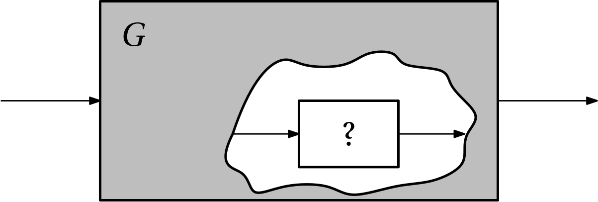
Figure 1: A subsystem is uncertain
A popular model for an uncertain subsystem is that of a transfer function \Delta(s), about which we know only that it is stable and that its magnitude is bounded by 1 \boxed
{\sup_{\omega}|\Delta(j\omega)|\leq 1,\;\;\Delta \;\text{stable}. }
Typically the uncertainty is higher at higher frequencies. This can be expressed by using some weighting function w(\omega). For later theoretical and computational purposes we approximate the real weighting function using a magnitude of a low-order rational stable transfer function W(s). That is, |W(j\omega)|\approx w(\omega) for \omega \in \mathbb R, that is for s=j\omega on the imaginary axis.
The ultimate transfer function model of the uncertainty is then \boxed{
W(s)\;\Delta(s),\quad \max_{\omega}|\Delta(j\omega)|\leq 1,\;\;\Delta\; \text{stable}. }
TipRational function W(s) distorts the phase but we do not care because \Delta(s) does it anyway
If you start worrying that by considering a rational function W(s) we inevitably distort the phase too (by \angle W(j\omega)), you can relax, because \Delta(s) does it anyway. The only responsibility of W(s) is to model the magnitude well.
\mathcal H_\infty norm of an LTI system
A useful concept for characterizing the magnitude of a transfer function is the \mathcal H_\infty norm. There are two (equivalent) definitions. One in the frequency domain, and the other in the time domain. We start with the former.
H-infinity norm of an LTI system interpreted in frequency domain
Definition 4 (\mathcal H_\infty norm of a SISO LTI system) For a stable LTI system modelled by the transfer function G with a single input and single output, the \mathcal H_\infty norm is defined as
\|G\|_{\infty} = \sup_{\omega\in\mathbb{R}}|G(j\omega)|.
NoteWhy supremum and not maximum?
Supremum is used in the definition because it is not guaranteed that the peak value of the magnitude frequency response is attained at a finite frequency. Consider, for example, the first-order system G(s) = \frac{s}{Ts+1}. The peak gain of 1/T is not attained at any finite frequency.
Having just defined the \mathcal H_\infty norm, the uncertainty model can be expressed compactly as \boxed{
W(s)\;\Delta(s),\quad \|\Delta(j\omega)\|\leq 1. }
Note\mathcal H_\infty as a space of functions
\mathcal H_\infty denotes a normed vector space of functions that are analytic in the closed extended right half plane (of the complex plane). In parlance of control systems, \mathcal H_\infty is the space of proper and stable transfer functions. Poles on the imaginary axis are not allowed. The functions do not need to be rational, but very often we do restrict ourselves to rational functions, in which case we typically write such space as \mathcal{RH}_\infty.
We now extend the concept of the \mathcal H_\infty norm to MIMO systems. The extension is perhaps not quite intuitive – certainly it is not computed as the maximum of the norms of individual transfer functions, which is what newcomers might guess.
Definition 5 (\mathcal H_\infty norm of a MIMO LTI system) For a stable LTI system modelled by a matrix transfer function \mathbf G with multiple inputs and/or multiple outputs, the \mathcal H_\infty norm is defined as
\|\mathbf G\|_{\infty} = \sup_{\omega\in\mathbb{R}}\bar{\sigma}(\mathbf{G}(j\omega))
where \bar\sigma is the largest singular value.
Here we include a short recap of singular values and singular value decomposition (SVD) of a matrix. Consider a matrix \mathbf M, possibly a rectangular one. It can be decomposed as a product of three matrices
\mathbf M = \mathbf U
\underbrace{
\begin{bmatrix}
\sigma_1 & & & &\\
& \sigma_2 & & &\\
& &\sigma_3 & &\\
\\
& & & & \sigma_n\\
\end{bmatrix}
}_{\boldsymbol\Sigma}
\mathbf V^{*}.
The two square matrices \mathbf V and \mathbf U are unitary, that is,
\mathbf V\mathbf V^*=\mathbf I=\mathbf V^*\mathbf V
and
\mathbf U\mathbf U^*=\mathbf I=\mathbf U^*\mathbf U.
The nonnegative diagonal entries \sigma_i \in \mathbb R_+, \forall i of the (possibly rectangular) matrix \Sigma are called singular values. Commonly they are ordered in a nonincreasing order, that is
\sigma_1\geq \sigma_2\geq \sigma_3\geq \ldots \geq \sigma_n.
It is also a common notation to denote the largest singular value as \bar \sigma, that is, \bar \sigma \coloneqq \sigma_1.
\mathcal{H}_{\infty} norm of an LTI system interpreted in time domain
We can also view the dynamical system with inputs and outputs as an operator G mapping from some chosen space of functions (signals) to another space of functions (signals). A popular model for these function/signal spaces are the spaces of square-integrable functions, denoted as \mathcal{L}_2, and sometimes interpreted as bounded-energy signals
G:\;\mathcal{L}_2\rightarrow \mathcal{L}_2.
It is a powerful fact that the induced operator norm is equal to the \mathcal{H}_{\infty} norm of the corresponding transfer function \boxed{
\|G\|_{\infty} = \sup_{u(\cdot)\in\mathcal{L}_2\setminus 0}\frac{\|y(\cdot)\|_2}{\|u(\cdot)\|_2}}.
Recall the definition of the \mathcal{L}_2 norm of a signal u(\cdot) (here we assume that the signal starts at time 0)
\|u(\cdot)\|_2 = \sqrt{\int_{0}^{+\infty}|u(t)|^2dt}.
In some cases the \mathcal{L}_2 norm of a signal u(\cdot) can be interpreted as (proportional to) the energy (when u(\cdot) is voltage, current, velocity, force, …). The system norm can then be interpreted as the worst-case energy gain of the system.
If the input or output signals are vector valued, we extend the definition to \boxed{
\|\mathbf G(s)\|_{\infty} = \sup_{\bm u(\cdot)\in\mathcal{L}_2\setminus 0}\frac{\|\bm y(\cdot)\|_2}{\|\bm u(\cdot)\|_2}},
in which the absolute value must be replaced by some norm, typically the Euclidean norm is used
\|\bm u(\cdot)\|_2 = \sqrt{\int_{0}^{+\infty}\|u(t)\|_2^2dt}.
ImportantScaling necessary for MIMO systems
Scaling of the model is necessary to get any useful info from MIMO models! See [1, Sec. 1.4], pages 5-8, which is contained in the online available part.
How does the uncertainty enter the model of the system?
Additive uncertainty
The transfer function of an uncertain system can be written as a sum of a nominal system and an uncertainty
G(s) = \underbrace{G_0(s)}_{\text{nominal model}}+\underbrace{W(s)\Delta(s)}_{\text{additive uncertainty}}.
The magnitude frequency response of the weighting filter W(s) then serves as an upper bound on the absolute error in the magnitude frequency responses
|G(j\omega)-G_0(j\omega)|<|W(j\omega)|\quad \forall \omega\in\mathbb R.
Multiplicative uncertainty
G(s) = (1+W(s)\Delta(s))\,G_0(s).
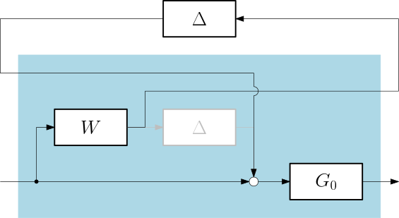
The block diagram interpretation is in
Figure 3: Multiplicative uncertainty
CautionFor SISO transfer functions no need to bother about the order of terms in the products
Sice we are considering SISO transfer functions, the order of terms in the products is not important. We will have to be more alert to the ordering of terms when we move to MIMO systems. We then have to distinguish between the input and output multiplicative uncertainties.
The magnitude frequency response of the weighting filter W(s) then serves as an upper bound on the relative error in the magnitude frequency responses \boxed
{\frac{|G(j\omega)-G_0(j\omega)|}{|G_0(j\omega)|}<|W(j\omega)|\quad \forall \omega\in\mathbb R.}
Example 2 (Uncertain first-order delayed system) We consider a first-order system with a delay described by
G(s) = \frac{k}{T s+1}e^{-\theta s}, \qquad 2\leq k,\tau,\theta,\leq 3.
We now need to choose the nominal model G_0(s) and then the uncertainty weighting filter W(s). The nominal model corresponds to the nominal values of the parameters, therefore we must choose these. There is no single correct way to do this. Perhaps the most intuitive way is to choose the nominal values as the average of the bounds. But we can also choose the nominal values in a way that makes the nominal system simple. For example, for this system with a delay, we can even choose the nominal value of the delay as zero, which makes the nominal system a first-order system without delay, hence simple enough for application of some basic linear control system design methods. Of course, the price to pay is that the resulting model of an uncertain system, which is actually a family (a set) of systems, contains even models that were not prescribed.
Figure 4: Magnitude of the relative error for a grid of parameters as a function of frequency
Now we need to find some upper bound on the relative error. Simplicity is a virtue here too, hence we are looking for a rational filter of very low order, say 1 or 2. Speaking of the first-order filter, one useful way to format it is
\boxed{
W(s) = \frac{\tau s+r_0}{(\tau/r_{\infty})s+1},}
where r_0 is uncertainty at steady state, 1/\tau is the frequency, where the relative uncertainty reaches 100%, r_{\infty} is relative uncertainty at high frequencies, often r_{\infty}\geq 2.
For our example, the parameters of the filter are in the code below and the frequency response follows.
Figure 5: (Approximate) upper bound on the magnitude of the relative error(s)
Obviously the filter does not capture the family of systems perfectly. It is now up to the control engineer to decide if this is a problem. If yes, if the control design should be really robust against all uncertainties in the considered set, some more complex (higher-order) filter is needed to described the uncertainty more accurately. The source code shows (in commented lines) one particular candidate, but in general the whole problem boils down to designing a stable filter with a prescribed magnitude frequency response.
We can also consider the configuration in which the uncertainty enters in a feedback manner as in Fig. 6 and Fig. 7.
Figure 6: Inverse additive uncertainty
Figure 7: Inverse multiplicative uncertainty
Through these feedback configurations we can also model unstable uncertain dynamics even if W and \Delta are stable.
Linear fractional transformation (LFT)
Finally, we are going to introduce a framework within which all the above described configurations can be expressed in a unified way. The framework is called linear fractional transformation (LFT). For a matrix \mathbf P sized (n_1+n_2)\times(m_1+m_2) and divided into blocks like
\mathbf P=
\begin{bmatrix}
\mathbf P_{11} & \mathbf P_{12}\\
\mathbf P_{21} & \mathbf P_{22}
\end{bmatrix},
and a matrix \mathbf K sized m_2\times n_2, the lower LFT of \mathbf P with respect to \mathbf K is
\boxed{
\mathcal{F}_\mathbf{l}(\mathbf P,\mathbf K) = \mathbf P_{11}+\mathbf P_{12}\mathbf K(\mathbf I-\mathbf P_{22}\mathbf K)^{-1}\mathbf P_{21}}.
If the matrices \mathbf P and \mathbf K are input-ouutput models (matrix transfer functions) of the plant and the controller, respectively, the LFT can be viewed as their interconnection in which not all plant inputs are used as control inputs and not all plant outputs are measured, as depicted in Fig. 8.
Figure 8: Lower LFT of \mathbf P with respect to \mathbf K
Similarly, for a matrix \mathbf N sized (n_1+n_2)\times(m_1+m_2) and a matrix \boldsymbol\Delta sized m_1\times n_1, the upper LFT of \mathbf N with respect to \mathbf K is
\boxed{
\mathcal{F}_\mathbf{u}(\mathbf N,\boldsymbol\Delta) = \mathbf N_{22}+\mathbf N_{21}\boldsymbol\Delta(\mathbf I-\mathbf N_{11}\boldsymbol\Delta)^{-1}\mathbf N_{12}}.
It can be viewed as a feedback interconnection of the nominal plant \mathbf N and the uncertainty block \boldsymbol\Delta, as depicted in Fig. 9.
Figure 9: Upper LFT of \mathbf N with respect to \boldsymbol \Delta
Here we already anticipated a MIMO uncertainty block. One motivation is explained in the next section on structured uncertainties, another one appears once we start formulating robust performance within the same analytical framework as robust stability.
NoteWhich is lower and which is upper is a matter of convention, but a useful one
Our usage of the lower LFT for a feedback interconnection of a (generalized) plant and a controller and the upper LFT for a feedback interconnection of a nominal system and and uncertainty is completely arbitrary. We could easily use the lower LFT for the uncertainty. But it is a convenient convention to adhere to. The more so that it allows for the combination of both as in the diagram Fig. 10 below, which corresponds to composition of the two LFTs.
Figure 10: Combination of the lower and upper LFT
Example 3 (Input multiplicative uncertainty formulated as an upper LFT) We advertized the LFT as a unifying modelling tool. Here comes an example. We consider the (input) multiplicative uncertainty and reformulate it as and upper LFT.
Figure 11: Input multiplicative uncertainty formulated as an upper LFT
We can read from Fig. 11 that the generalized plant \mathbf P is modelled by the matrix transfer function
\mathbf P =
\begin{bmatrix}
0 & W\\
G_0 & G_0
\end{bmatrix}.
Structured frequency-domain uncertainty
Not just a single \Delta(s) but several \Delta_i(s), i=1,\ldots,n are considered. In the upper LFT framework, all the individual \Delta_is are collected into a single overall \boldsymbol \Delta, which then exhibits a diagonal structure.
\boldsymbol\Delta =
\begin{bmatrix}
\Delta_1& 0 & \ldots & 0\\
0 & \Delta_2 & \ldots & 0\\
\vdots\\
0 & 0 & \ldots & \Delta_n
\end{bmatrix},
with each \Delta_i satisfying the usual condition
\|\Delta_i\|_{\infty}\leq 1, \; i=1,\ldots, n.
Example 4 (Several uncertain parameters approximated by multiple \Delta terms) We consider a model of a system
G(s;p_1,p_2) = \frac{1}{(s+p_1)(s+p_2)},
where p_1 and p_2 are uncertain parameters satisfying p_1\in[0.9,1.1], p_2\in[3,5].
After choosing the nominal values of the paratemeters to be, say, in the middle of the intervals, we can express the uncertain parameters as
p_1 = 1+0.1\delta_1,\quad p_2 = 4+\delta_2,
where the uncertain real parameters satisfy |\delta_1|\leq 1 and |\delta_2|\leq 1. We can then model the uncertain system as in Fig. 12.
Figure 12: The two-real-pole system with uncertain location of poles modelled as two integrators with uncertain gain in the feedback
We can then isolate the uncertain parameters as in Fig. 13.
Figure 13: Modification of Fig. 12 so that the uncertain parameters are isolated
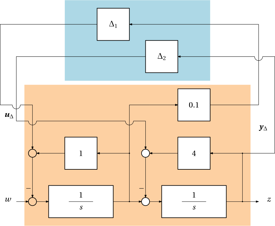
And finally we can manipulate the block diagram in the form of a lower LFT as in Fig. 14. Note that we have approximated the uncertain real parameters \delta_1 and \delta_2 conservatively by uncertain complex parameters \Delta_1 and \Delta_2. This surely introduces some conservatism into the model.
Figure 14: Reformatting Fig. 13 into the lower LFT (with the uncertain real parameters \delta_1 and \delta_2 approximated conservatively by uncertain complex parameters \Delta_1 and \Delta_2)
The blue block in Fig. 14 is the uncertain block \bm\Delta = \begin{bmatrix}\Delta_1 & 0\\ 0& \Delta_2\end{bmatrix}. The orange block is the nominal system \mathbf N, which has three inputs and three outputs. The last two inputs and the last two outputs are related to the uncertainty, we label them \bm u_\Delta and \bm y_\Delta, respectively. The matrix transfer function is
S. Skogestad and I. Postlethwaite, Multivariable Feedback Control: Analysis and Design, 2nd ed. Wiley, 2005. Available: https://folk.ntnu.no/skoge/book/