Robustness analysis for unstructured uncertainty
When we introduced the concept of robustness, we only vaguely hinted that it is always related to some property of interest. Now comes the time to specify these two properties:
Definition 1 (Robust stability) Guaranteed stability of the closed feedback loop with a given controller for all admissible (=considered apriori) deviations of the model from the reality.
Definition 2 (Robust performance) Robustness of some performance characteristics such as steady-state regulation error, attenuation of some specified disturbance, insensitivity to measurement noise, fast response, ….
Internal stability
Before we start discussing robust stability, we need to discuss one fine issue related to stability of a nominal system. We do it through the following example.
Example 1 (Internal stability) Consider the following feedback system with a nominal plant G(s) and a nominal controller K(s).

The question is: is this closed-loop system stable? We determine stability by looking at the denominator of a closed-loop transfer function. But which one? There are several. Perhaps the most immediate one is the transfer function from the reference r to the plant output y. With the open-loop transfer function L(s) = G(s)K(s) = \frac{s-1}{s+1} \frac{k(s+1)}{s(s-1)} = \frac{k}{s}, the closed-loop transfer function is T(s) = \frac{\frac{k}{s}}{1+\frac{k}{s}} = \frac{k}{s+k}, which is perfectly stable. But note that for practical purposes, all possible closed-loop transfer functions must be stable. How about the one from the output disturbance d to the plant output y? S(s) = \frac{1}{1+\frac{k}{s}} = \frac{s}{s+k}, which is stable too. Doesn’t this indicate that we can stop worrying? Not yet. Consider now the closed-loop transfer function from the reference r to the control u. The closed-loop transfer function is K(s)S(s) = \frac{\frac{k(s+1)}{s(s-1)}}{1+\frac{k}{s}} = \frac{k(s+1)}{{\color{red}(s-1)}(s+k)}.
Oops! This closed-loop transfer function is not stable.
The culprit here is our cancelling the zero in the right half-plane (RHP) with an unstable pole in the controller. But let’s emphasize that the trouble is not in imperfectness of this cancellation due to numerical errors. The trouble is in the very cancelling the zero in the RHP by the controller. Identical problem would arise if an unstable pole of the plant is cancelled by the RHP zero of the controller as we can see by modifying the assignment accordingly.
The example taught (or reminded) us that in order to guarantee stability of all closed-loop transfer functions, no cancellation of poles and zeros in the right half plane is allowed. The resulting closed-loop system is then called internally stable. Checking just (arbitrary) one closed-loop transfer function for stability is then enough to conclude that all of them are stable too.
Robust stability for a multiplicative uncertainty
We consider a feedback system with a plant G(s) and a controller K(s), where the uncertainty in the plant modelled as multiplicative uncertainty, that is, G(s) = (1+W(s)\Delta(s))\,G_0(s).
The technique for analyzing closed-loop stability is based on Nyquist criterion. Instead of analyzing the Nyquist plot for the nominal plant G_0(s), we analyze the Nyquist plot for the uncertain plant G(s). The corresponding open-loop transfer function is L(s) = G(s)K(s) = (1+W(s)\Delta(s))\,G_0(s)K(s) = L_0(s) + W(s)L_0(s)\Delta(s).
When trying to figure out the conditions under which this family of Nyquist curves avoids the point -1, it is useful to interpret the last equation at a given frequency \omega as a disc with the center at L_0(j\omega) and the radius W(j\omega)L_0(j\omega). To see this, note that \Delta(j\omega) represents a complex number with a magnitude up to one, and with an arbitrary angle.
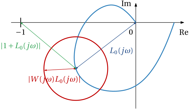
The geometric formulation of the condition is then that the distance from -1 to the nominal Nyquist plot of L_0(j\omega) is greater than the radius W(j\omega)L_0(j\omega) of the disc centered at the nominal Nyquist curve With the distance from the point -1 to the nominal Nyquist plot of L_0(s) evaluated at a particular frequency \omega a |-1-L_0(j\omega)| = |1+L_0(j\omega)|, the condition can be written as
|W(j\omega)L_0(j\omega)| < |1+L_0(j\omega)|, \;\forall \omega.
Dividing both sides by 1+L_0(j\omega) we get \frac{W(j\omega)L_0(j\omega)}{1+L_0(j\omega)} < 1, \;\forall \omega.
But recalling the definition of the complementary sensitivity function, and dividing both sides by W, we can rewrite the condition as \boxed {|T_0(j\omega)| < 1/|W(j\omega)|, \;\; \forall \omega.}
This condition has clear interpretation in terms of the magnitude of the complementary sensitivity function – it must be smaller than the reciprocal of the magnitude of the uncertainty weight at all frequencies.
Finally, we can also invoke the definition of the \mathcal H_\infty norm and reformulate the condition as \boxed {\|WT\|_{\infty}< 1.}
To appreciate usefulness of the this format of the robust stability condition beyond mere notational compactness, we mention that \mathcal H_\infty norm of an LTI system can be reliably computed. Robust stability can then be then checked by computing a single number.
In fact, it is even better than that – there are methods for computing a feedback controller that minimizes the \mathcal H_\infty norm of a specified closed-loop transfer function, which suggests an optimization-based approach to design of robustly stabilizing controllers. We are going to build on this in the next chapter. But let’s stick to the analysis for now.
Robust stability for an LFT – small gain theorem
We now aim at developing a similar robust stability condition for the (upper) LFT, as in Fig. 3.

The term corresponding to the nominal closed-loop system is structured into blocks. It is only the N_{11} block that captures the interaction with the uncertainty in the model, that is why we are going to analyze the corresponding feedback loop. For convenience we rename this block as M \coloneqq N_{11}, and the open-loop transfer function is then M \Delta. Following the same Nyquist criterion based reasoning as before, that is, asking for the conditions under which this open-loop transfer function does not touch the point -1, while the \Delta term can introduce an arbitrary phase, we arrive at the following robust stability condition for the LFT \boxed {|M(j\omega)|<1,\;\;\forall \omega.}
Invoking the definition of the \mathcal H_\infty norm, we can rewrite the condition compactly as \boxed {\|M\|_{\infty}<1.}
Once again, the formulation as an inequality over all frequencies can be useful for visualization and interpretation, while the inequality with the \mathcal H_\infty norm can be used for computation and optimization.
This condition of robust stability belongs to the most fundamental results in control theory. It is known as the small gain theorem.
Small gain theorem works for a MIMO uncertainty \boldsymbol \Delta and a block \mathbf N_{11} (or \mathbf M) too \|\mathbf M\|_{\infty}<1.
But we discuss in the next section that it is typically too conservative as the \boldsymbol \Delta block has typically some (block diagonal) structure, which should be exploited. But more on this in the section dedicated to structured uncertainty.
Nominal performance
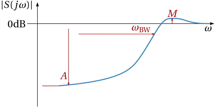
Having discussed stability (and its robustness), it is now time to turn to performance (and its robustness). Performance can mean different things for different people, and it can be specified in a number of ways, but we would like to formulate performance requirements in the same frequency domain setting as we did for (robust) stability. Namely, we would like to specify the performance requirements in terms of the frequency response of some closed-loop transfer function. The sensitivity function seems to be a natural choice for this purpose. It turns out that by imposing upper bound constraints on |S(j\omega)| (actually |S_0(j\omega)| as we now focus on the nominal case with no uncertainty) we can specify a number of performance requirements:
- Up to which frequency the feedback controller attenuates the disturbance, that is, the bandwidth \omega_\mathrm{BW} of the system.
- How much the feedback controller attenuates the disturbances over the bandwidth.
- How does it behave at very low frequencies, that is, how well it regulates the steady-state error.
- What is the maximum amplification of the disturbance, that is, the resonance peak.
These four types of performance requirements can be pointed at in Fig. 4 below.
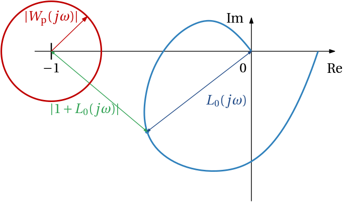
But these requirements can also be compactly expressed throug the performance weighting filter W_\mathrm{p}(s) as \boxed {|S_0(j\omega)| < 1/|W_\mathrm{p}(j\omega)|,\;\;\forall \omega,} \tag{1}
where S_0 = \frac{1}{1+L_0} is the sensitivity function of the nominal closed-loop system. which can be compactly written as \boxed {\|W_\mathrm{p}S_0\|_{\infty}<1.}
Simple (low-order) weighting filter usually suffices, such as W_{\mathrm{p}}(s) = \frac{s/M+\omega_\mathrm{B}^*}{s+\omega_\mathrm{B}^*A}, or W_\mathrm{p}(s) = \frac{(s/\sqrt{M}+\omega_\mathrm{B}^*)^2}{(s+\omega_\mathrm{B}^*\sqrt{A})^2}, where M is allowed peak in the sensitivity function, \omega_\mathrm{B}^* is the bandwidth, that is, the frequency up to which the disturbance is attenuated, and A is the attenuation of the disturbance at low frequencies. In particular, if A=0, the steady-state error is zero.
It lends some insight if we visualize this condition in the complex plane. First, recall that S_0 = \frac{1}{1+L_0}. Eq. 1 then translates to |W_\mathrm{p}(j\omega)|<|1+L_0(j\omega)|\;\;\forall \omega, which can be visualized as in Fig. 5.
Robust performance for a multiplicative uncertainty
So far we have the condition of robust stability and the condition of nominal performance. Simultaneous satisfaction of both gives… just robust stability and nominal performance. Robust performance obviously needs a stricter condition. We visualize it in Fig. 6.
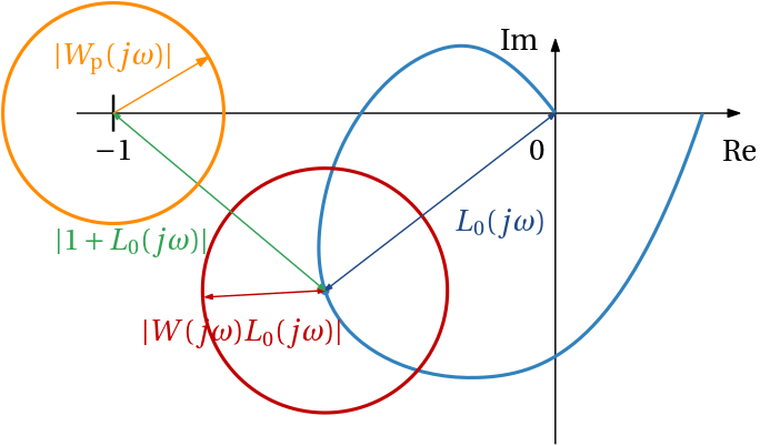
In words, the two circles, one corresponding to the uncertainty, the other corresponding to the performance specifications, must not even touch. This we can express algebraically as \boxed{ |W_\mathrm{p}(j\omega)S_0(j\omega)| + |W(j\omega)T_0(j\omega)| < 1\;\;\forall \omega.} \tag{2}
How about rewriting this condition in terms of the \mathcal H_\infty norm? It appears this is not as straightforward as in the previous two cases of robust stability and nominal performance. But there is something we can do. We consider the following artificial/auxilliary/augmented closed-loop transfer function that we call mixed sensitivity function \begin{bmatrix} W_\mathrm{p}S_0\\ WT_0 \end{bmatrix}.
Its \mathcal H_\infty norm can be written as \left\| \begin{bmatrix} W_\mathrm{p}S\\ WT \end{bmatrix} \right\|_{\infty} = \sup_{\omega\in\mathbb{R}}\sqrt{|W_\mathrm{p}(j\omega)S(j\omega)|^{2}+|W(j\omega)T(j\omega)|^{2}}.
This can be seen by using the known relation between singular values and eigenvalues. Consider a matrix \mathbf A \in \mathbb R^{n\times m}, it holds that \sigma_i(\mathbf A) = \sqrt{\lambda_i(\mathbf A^\top \mathbf A)}, where \sigma_i is the i-th singular value of a matrix, and \lambda_i is the i-th eigenvalue. Although this is not how singular values are computed numerically (there are more reliable ways), we can use this result for our theoretical derivation. Note that if \mathbf A is a one-column matrix (a column vector), the product \mathbf A^\top \mathbf A is a scalar; it is equal to the square of the Euclidean norm of \mathbf A. Hence, the only (nonzero) singular value of a one-column matrix is the Euclidean norm of the one-column \mathbf A.
We have just learnt that \left\| \begin{bmatrix} W_\mathrm{p}S\\ WT \end{bmatrix} \right\|_{\infty} = \sup_{\omega\in\mathbb{R}} \left\| \begin{bmatrix} W_\mathrm{p}(j\omega)S(j\omega)\\ W(j\omega)T(j\omega) \end{bmatrix} \right\|_{2}. \tag{3}
In the above equation, the norm on the left is a norm of a transfer function, the norm on the right is a norm of a constant vector (evaluated at a particular frequency \omega). In order to emphasize it, some authors use the notation \|\cdot\|_{\mathcal H_\infty} to distinguish the \mathcal H_\infty norm of a transfer function from the \infty- (also called max-) norm \|\cdot\|_\infty of a constant vector.
The condition of robust performance in Eq. 2 uses the 1-norm of a vector evaluated at a particular frequency \omega. We can rewrite it as \sup_{\omega\in\mathbb{R}} \left\| \begin{bmatrix} W_\mathrm{p}(j\omega)S(j\omega)\\ W(j\omega)T(j\omega) \end{bmatrix} \right\|_{1} < 1. \tag{4}
Now what? The condition of robust performance enforces frequency-wise upper bound on the 1-norm, but the \mathcal H_\infty system norm can be interpreted as a frequency-wise upper bound on the 2-norm. The good news is that these norms are related. For notational convenience, we consider just some vector \bm x = \begin{bmatrix} x_1 \\ x_2 \end{bmatrix}. Here come definitions of three most popular vector norms: \|\bm x\|_2 = \sqrt{x_1^2+x_2^2},\quad \|\bm x\|_1 = |x_1| + |x_2|,\quad \|\bm x\|_{\infty} = \max\{|x_1|,|x_2|\}.
These definitions are also visualized in Fig. 7 a.
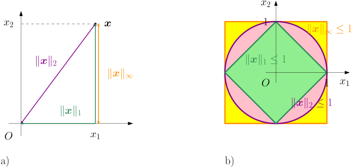
From Fig. 7 b, we can deduce the following inequalities \|\bm x\|_2 \leq \|\bm x\|_1\leq \sqrt{2}\|\bm x\|_2.
Therefore RP condition in the SISO case can be formulated as \boxed {\left\| \begin{bmatrix} W_\mathrm{p}S_0\\ WT_0 \end{bmatrix} \right\|_{\infty} <\frac{1}{\sqrt{2}}.}
In the MIMO case we do not have a useful upper bound, but at least we have received a hint that it may be useful to minimize the \mathcal H_\infty norm of the mixed sensitivity function. This observation will directly lead to a control design method.
Robust stability for MIMO multiplicative uncertainty
Back to the robust stability analysis. For MIMO systems, the general model of uncertainty is \mathbf E = \mathbf W_2\boldsymbol \Delta \mathbf W_1,\;\ \|\boldsymbol\Delta\|_{\infty}\leq 1, and the robust stability condition depends on whether the uncertainty is modelled as the output or at the input of the plant.
Say, the model of the uncertainty is just \mathbf E = \boldsymbol \Delta \mathbf W. For the output multiplicative uncertainty, the model of the uncertain plant is \mathbf G = \mathbf G_0 (\mathbf I+\boldsymbol \Delta \mathbf W), and the lower-upper LFT is in Fig. 8
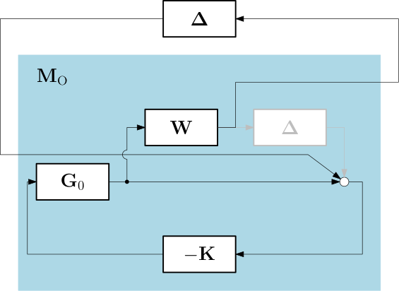
The transfer function of the M block is \mathbf M_\mathrm{O} = -\mathbf W\mathbf G_{0}\mathbf K(\mathbf I+\mathbf G_{0}\mathbf K)^{-1} = -\mathbf W \mathbf T_\mathrm{O}.
Similarly, for the input multiplicative uncertainty, the model of the uncertain plant is \mathbf G = (\mathbf I+\boldsymbol \Delta \mathbf W)\mathbf G_0, the lower-upper LFT is in Fig. 8
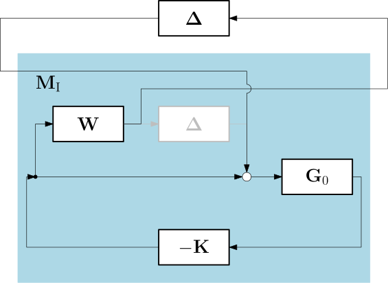
and the transfer function of the M block is \mathbf M_\mathrm{I} = -\mathbf W\mathbf K\mathbf G_{0}(\mathbf I+\mathbf K\mathbf G_{0})^{-1} = -\mathbf W \mathbf T_\mathrm{I}.
Robust performance as robust stability with structured uncertainty
A useful observation is that we can formulate the robust performance condition as a robust stability condition with a structured uncertainty. First, note that by refering to Fig. 10, the robust performance requirement can be state as: make the \mathcal H_\infty norm of the closed-loop transfer function from the disturbance d to the output d” small (smaller than one).
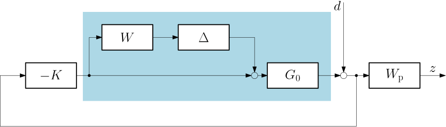
But we have already learnt that the condition on the \mathcal H_\infty norm can be interpreted as a condition on the robust stability of the given system and some \Delta block. We introduce such artificial uncertainty block \Delta_\mathrm{p} here and plug it into the feedback loop with the whole system as in Fig. 11.
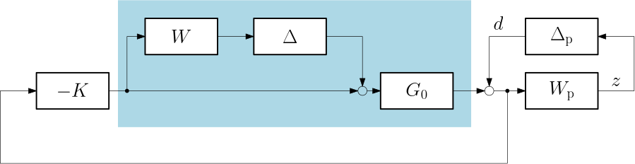
We emphasize that it does not represent any uncertainty but ruther serves to expresses the robust performance requirement, albeit indirectly via reformulating the whole problem as robust stability with a single augmented uncertainty block \bm \Delta^\mathrm{aug} = \begin{bmatrix} \Delta & 0\\ 0 & \Delta_\mathrm{p} \end{bmatrix}.
In this very special case of a system with a multiplicative uncertainty, we already showed how to write down the robust performance condition, hence it might not be clear why we have just reformulated the problem in a way that calls for the ability to analyze robust stability with a structured uncertainty (which we do not yet have). But still, it shows the very essential idea that we are going to use later within some more complicated setups, such as the ones with the original uncertainty block \bm \Delta already structured.