Optimal control with a free final time
Free final time and free final state
We start by considering the optimal control problem where both the final time and the state at this final time are subject to optimization. Later we will consider modification in which the final state is constrained in one way or another.
Free end in calculus of variations
We adhere to our style of developing the results within the framework of calculus of variations first. The problem we are going to solve is visualized in Fig. 1.
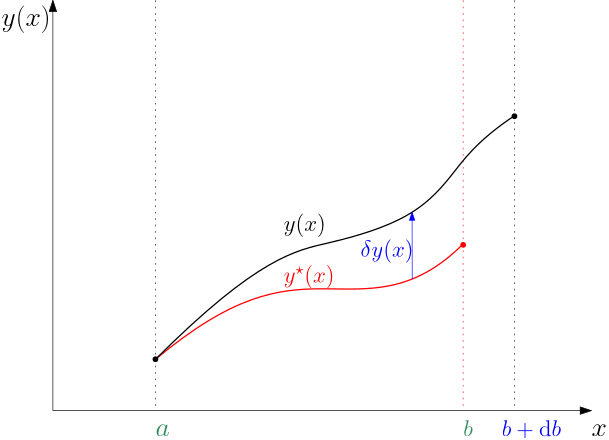
The key trick is that stretching or shrinking the interval of the independent variable is done by perturbing the stationary value of the right end b of the interval in proportion to the same \alpha we use to perturb the functions y and y'. That is, b is perturbed by \Delta b = \alpha \Delta x and the perturbed cost functional is then J(y^\star+{\color{blue}\alpha} \eta) = \int_a^{{\color{red}b}+{\color{blue}\alpha}\Delta x} L(x,y^\star +{\color{blue}\alpha} \eta,(y^\star )'+{\color{blue}\alpha} \eta')\text{d}x.
We do not use b^\star for the stationary value of the right end of the interval in favour of notational simplicity. Admittedly, this comes at the cost of losing a bit of consistency in the notation.
Note that we have a minor technical problem here since the function y^\star is only defined on the interval [a,b]. But there is an easy fix: we define a continuation of the function to the right of b in the form of a linear approximation given by the derivative of y^\star at b. We will exploit it in a while.
Now, in order to find the variation \delta J, we can proceed by fitting the Taylor’s expansion of the above perturbed cost function to the general Taylor’s expansion and identifying the first-order term in \alpha. Equivalently, we can use the earlier stated fact that \delta J = \left.\frac{\text{d}}{\text{d}\alpha}J(y^\star +\alpha\eta)\right|_{\alpha=0}\alpha.
In order to find the derivative, we observe that the variable with respect to which we are differentiating is included in the upper bound of the integral. Therefore we cannot just change the order of differentiation and integration. This situation is handled by the well-known Leibniz rule for differentiation under the integral sign (look it up yourself in the full generality). In our case it leads to \left.\frac{\text{d}}{\text{d}\alpha}J(y^\star +\alpha\eta)\right|_{\alpha=0} = \int_a^{b} \left( L_y-\frac{\text{d}}{\text{d}x}L_{y'}\right)\eta(x)\text{d}x + \left.L_{y'}\right|_{b}\eta(b) + \left.L\right|_{b}\Delta x, which after multiplication by \alpha gives the variation of the functional \boxed{ \delta J = \int_a^{b} \left( L_y-\frac{\text{d}}{\text{d}x}L_{y'}\right)\delta y(x)\text{d}x + \left.L_{y'}\right|_{b}\delta y(x) + \left.L\right|_{b}\underbrace{\Delta x\alpha}_{\Delta b},} where the first two terms on the right are already known to us, and the only new term is the third one. The reasoning now is pretty much the same as it was in the fixed-interval free-end case. We argue that among the variations \delta y there are also those that vanish at b, hence the conditions must be satisfied even if the last two terms are zero. But then the integral must be zero, which gives rise to the familiar Euler-Lagrange equation. The last two terms must together be zero and it does not hurt to rewrite them in a complete notation to dispell any ambiquity \boxed{ \left.\frac{\partial L(x,y(x),y'(x))}{\partial y'}\right|_{x=b}\delta y(b) + \left.L(x,y(x),y'(x))\right|_{x=b}\Delta b = 0.} \tag{1}
Now, in order to get some more insight into the above condition, the relation between the participating objects can be further explored. We will do it using Fig. 1 but we augment it a bit with a few labels, see Fig. 2 below.
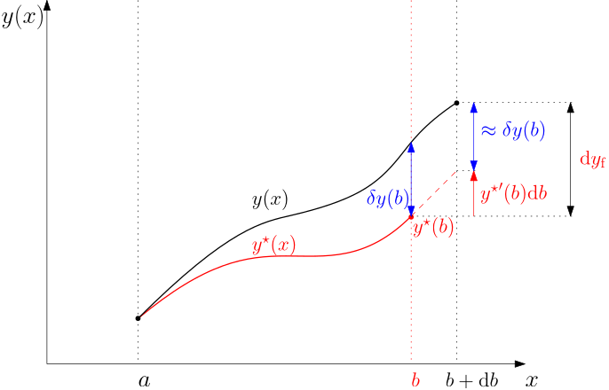
Note that we have included a brand new label here, namely, \mathrm{d}y_\mathrm{f} for the perturbation of the value of the function y() at the end of the interval (taking into consideration that the length of the interval can change as well). We can now write y^\star (b+\Delta b) + \delta y(b+\Delta b) = y^\star (b)+\mathrm{d}y_\mathrm{f}, which after approximating each term with the first two terms of its Taylor expansion gives \cancel{y^\star (b)}+{y^\star }'(b)\Delta b + \delta y(b)+\cancel{\delta'(b) \Delta b} = \cancel{y^\star (b)}+\mathrm{d}y_\mathrm{f}.
Note that the third product on the left can be neglected since it contains two terms that are both of order one in the perturbation variable \alpha. In other words, we approximate \delta y(b+\Delta b) by \delta y(b). In addition, the term y^\star (b) can be subtracted from both sides. From what remains after these cancelations, we can conclude that {y^\star }'(b)\Delta b + \delta y(b) = \mathrm{d}y_\mathrm{f}, or, equivalently, \delta y(b) = \mathrm{d}y_\mathrm{f} - {y^\star }'(b)\Delta b.
We will now substitute this into the general form of the boundary equation in () L_{y'}(b,y(b),y'(b))\,\left[\mathrm{d}y_\mathrm{f} - {y^\star }'(b)\Delta b\right] + L(b,y(b),y'(b))\Delta b = 0. \tag{2}
Collecting now the terms with the two perturbation variables \mathrm d y_\mathrm{f} and \Delta b, we reformat the above expression into \boxed{ L_{y'}(b,y(b),y'(b))\mathrm{d}y_\mathrm{f} + \left[L(b,y(b),y'(b))-L_{y'}(b,y(b),y'(b)) {y^\star }'(b)\right]\Delta b = 0.} \tag{3}
Now, since \mathrm d y_\mathrm{f} and \Delta b are assumed independent, the corresponding terms must be simultaneously and independently equal zero, that is, \begin{aligned} L_{y'}(b,y(b),y'(b)) &= 0,\\ L(b,y(b),y'(b))-L_{y'}(b,y(b),y'(b)) {y^\star }'(b) &= 0. \end{aligned}
Note that the first condition actually constitutes n scalar conditions whereas the second one is just a scalar condition itself, hence, n+1 boundary conditions.
Optimal control setting
Let’s now switch back to the optimal control setting with t as the independent variable. Recall that the optimal control problem is \min_{\bm x(),\bm u(),t_\mathrm{f}} \left[\phi(\bm x(t_\mathrm{f}))+\int_{t_\mathrm{i}}^{t_\mathrm{f}}L(\bm x,\bm u,t)\text{d}t\right]. subject to \dot{\bm x}(t)= \mathbf f(\bm x,\bm u,t),\qquad \bm x(t_\mathrm{i}) = \mathbf x_\mathrm{i}.
We have already seen that the integrand of the augmented cost function now contains not only the term that corresponds to the Lagrange multiplier but also the term that penalizes the state at the final time, that is, L^\mathrm{aug}(\bm x,\bm u,\boldsymbol \lambda, t) = L(\bm x,\bm u,t) + \underbrace{\frac{\partial \phi}{\partial t} + (\nabla_{\bm x}\phi)^\top \frac{\mathrm d \bm x }{\mathrm d t}}_{\frac{\mathrm d \phi(\bm x(t), t)}{\mathrm d t}} + \boldsymbol{\lambda}^\top (\mathbf f(\bm x,\bm u,t)-\dot{\bm{x}}). \tag{4}
We then rewrite the boundary conditions Eq. 3 as \boxed{ \left.(\nabla_\mathbf{x}\phi-\boldsymbol \lambda)\right|_{t=t_\mathrm{f}}^\top \mathrm{d}\mathbf{x}_\mathrm{f} + \left.\left(L+\frac{\partial \phi}{\partial t}+\boldsymbol \lambda^\top f(\bm x, \bm u, t)\right)\right|_{t=t_\mathrm{f}}\mathrm d t_\mathrm{f}.}
Since here we assume that the final time and the state at the final time are independent, this single conditions breaks down into two boundary conditions
\begin{aligned} \nabla_\mathbf{x}\phi(x(t_\mathrm{f}),t_\mathrm{f})-\boldsymbol \lambda(t_\mathrm{f}) &=0\\ L(x(t_\mathrm{f}),u(t_\mathrm{f}),t_\mathrm{f})+\frac{\partial \phi(\mathbf{x}(t_\mathrm{f}),t_\mathrm{f})}{\partial t}+\boldsymbol \lambda^\top (t_\mathrm{f}) f(\bm x(t_\mathrm{f}), \bm u(t_\mathrm{f}), t_\mathrm{f}) &=0. \end{aligned}
The first one is actually representing n scalar conditions, the second one is just a single scalar condition. Hence, altogether we have n+1 boundary conditions.
Here we commit the common abuse of notation in writing the functions to be differentiated as explicitly dependent on t_\mathrm{f} such as in \frac{\partial \phi(\mathbf{x}(t_\mathrm{f}),t_\mathrm{f})}{\partial t}. Instead, we should perhaps keep writing it as \left.\frac{\partial \phi(\mathbf{x}(t),t)}{\partial t}\right|_{t=t_\mathrm{f}}, but the formulas then look rather cluttered.
Let’s try to get some more insight into this. We assume now that the term penalizing the state at the final time does not explicitly depend on time, that is, \frac{\partial \phi}{\partial t}=0. Then the boundary condition modifies to \left.(\nabla_\mathbf{x}\phi-\boldsymbol \lambda)\right|_{t=t_\mathrm{f}}^\top \mathrm{d}\mathbf{x}_\mathrm{f} + \left.\left(L+\boldsymbol \lambda^\top f(\bm x, \bm u, t)\right)\right|_{t=t_\mathrm{f}}\mathrm d t_\mathrm{f}, which can be rewritten as \left.(\nabla_\mathbf{x}\phi-\boldsymbol \lambda)\right|_{t=t_\mathrm{f}}^\top \mathrm{d}\mathbf{x}_\mathrm{f} + \left.H(\bm x,\bm u,\boldsymbol \lambda,t)\right|_{t=t_\mathrm{f}}\mathrm d t_\mathrm{f}, which, in turn, enforces the scalar boundary condition (on top of those other n conditions) \boxed{ \left.H(\bm x(t),\bm u(t),\boldsymbol \lambda(t),t)\right|_{t=t_\mathrm{f}}\mathrm d t_\mathrm{f}=0}.
This observation is worth memorizing – for a free-final-time optimal control problem, Hamiltonian vanishes at the end of the time interval.
Let’s now add one more observation. We could have mentioned it even in the previous lecture since it is a general property of a Hamiltonian evaluated along the optimal solution – the total derivative of a Hamiltonian with respect to time, when evaluated along the solution, is equal to its partial derivative with respect to time: \frac{\mathrm{d}H}{\mathrm{d}t} = \underbrace{\frac{\partial H}{\partial \bm x}}_{-\dot{\boldsymbol \lambda}}\frac{\mathrm{d}\bm x}{\mathrm{d}t} + \underbrace{\frac{\partial H}{\partial \boldsymbol \lambda}}_{\dot{\mathbf{x}}}\frac{\mathrm{d}\boldsymbol \lambda}{\mathrm{d}t} + \underbrace{\frac{\partial H}{\partial \bm u}}_{0}\frac{\mathrm{d}\bm u}{\mathrm{d}t} + \frac{\partial H}{\partial t} = \frac{\partial H}{\partial t}.
Now, if neither the system equations nor the optimal control cost function depend explicitly on time, that is, if \frac{\partial H}{\partial t}=0, the Hamiltonian remains constant along the optimal trajectory, that is, \boxed{ H(\bm x(t),\bm u(t),\boldsymbol \lambda(t)) = \mathrm{const.}\quad \forall t}
Combined with the previous result (boundary value of H at the end of the free time interval is zero), we obtain the powerful conclusion that the Hamiltonian evaluated along the optimal trajectory is always zero in the free-final-time scenario: \boxed{ H(\bm x(t),\bm u(t),\boldsymbol \lambda(t)) = 0\quad \forall t}
This is an insightful piece of information. Since some (numerical) techniques for optimal control are based on iterative minimization of a Hamiltonian, here we already know the minimum value.
Free final time but the final state on a prescribed curve
Calculus of variations setting
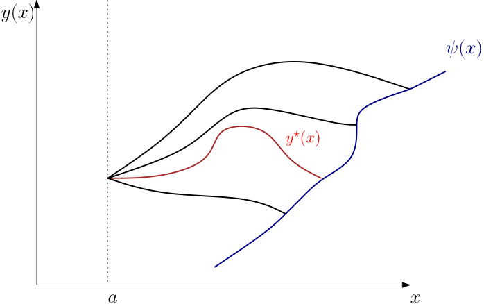
We will now investigate the case when the final value of the solution y(x) is to be on the curve described by \psi(x), that is y^\star (b+\Delta b) + \delta y(b+\Delta b) = \psi(b+\Delta b). \tag{5}
This corresponds to the situation depicted in Fig. 3.
We already discussed the terms on the left. What is new here is the term on the right. It can also be approximated by the first two terms in the Taylor’s expansion \psi(b+\Delta b) = \psi(b) + \psi'(b)\Delta b.
Therefore, we can expand Eq. 5 into \cancel{y^\star (b)} + (y^\star )'(b)\Delta b + \delta y(b) = \underbrace{\cancel{y^\star (b)}}_{\psi(b)}+\psi'(b)\Delta b, from which we can express \delta y(b) as \delta y(b) = \psi'(b)\Delta b - (y^\star )'(b)\Delta b, and substitute to the boundary condition Eq. 1, which after cancelling the common \Delta b term yields \boxed{ L_{y'}(b,y(b),y'(b))\,\left[\psi'(b)-y'(b)\right] + L(b,y(b),y'(b)) = 0.} \tag{6}
This is just one scalar boundary conditions. But the original n conditions that the state that y(x) = \psi(x) at the right end of the interval must be added. Altogether, we have n+1 boundary conditions.
The above single equation Eq. 6 is called transversality condition for the reason to be illuminated by the next example.
Example 1 To get an insight, consider again the minimum distance problem. This time we want to find the shortest distance from a point to a curve given by \psi(x). The answer is intuitive, but let us see what our rigorous tools offer here. The EL equation stays intact, therefore we know that the shortest path is a line. It starts at (a,0) but in order to determine its end, we need to invoke the other boundary condition. Remember that the Lagrangian is L = \sqrt{1+(y')^2}\text{d}x and L_{y'} = \frac{y'}{\sqrt{1+(y')^2}}\text{d}x.
The transversality condition boils down to 1+y'(b)\psi'(b)=0, which can also be visualized using vectors in the plane \begin{bmatrix}1 & y'(b)\end{bmatrix}\, \begin{bmatrix}1 \\ \psi'(b)\end{bmatrix} = 0.
The interpretation of this result is that our desired curve y hits the target curve \psi in a perpendicular (transverse) direction.
Understanding the boundary conditions is crucial. Let us have yet another look at the result just derived. It can be written as \boxed{ \left.L_{y'}\psi'\right|_{b} - \left.H\right|_{b} = 0.}
It follows that for a free length of the interval and fixed value of the variable at the end of the interval, in which \psi(x) = c,\; c\in\mathbb R, the transversality condition simplifies to \boxed{ H(b) = 0.}
Optimal control setting
Once again, let’s recall that the optimal control problem is \min_{\bm x(\cdot),\bm u(\cdot),t_\mathrm{f}} \left[\phi(\bm x(t_\mathrm{f}))+\int_{t_\mathrm{i}}^{t_\mathrm{f}}L(\bm x,\bm u,t)\text{d}t\right]. subject to \begin{aligned} \dot{\bm x}(t)&= \mathbf f(\bm x,\bm u,t),\\ \bm x(t_\mathrm{i}) &= \mathbf x_\mathrm{i}\\ \bm x(t_\mathrm{f}) &= \boldsymbol \psi(t_\mathrm{f}). \end{aligned}
Translating the above derived transversality condition from the domain (and notation) of calculus of variations to the optimal control setting gives \boxed{ \left.(\nabla_\mathbf{x}\phi-\boldsymbol \lambda)^\top \dot{\boldsymbol\psi}(t) + L+\frac{\partial \phi}{\partial t}+\boldsymbol \lambda^\top \mathbf f(\bm x, \bm u, t)\right|_{t=t_\mathrm{f}}=0.}
Of course, on top of this single condition, the 2n boundary conditions shown above must be added \boxed{ \begin{aligned} \bm x(t_\mathrm{i}) &= \mathbf x_\mathrm{i},\\ \bm x(t_\mathrm{f}) &= \boldsymbol \psi(t_\mathrm{f}). \end{aligned}}
Note that the video linked below, which covers the material of this lecture, uses the other convention for the control Hamiltonian, the one leading to the maximization of the Hamiltonian. Other than that, the (structure of the) results is the same.