We now consider an extension to the standard LQR problem, namely, the plant is subject to random disturbances and the initial state is also random. The question for which we seek an answer is: how does this affect the design of the optimal LQR controller? The question surely makes sense in both discrete- and continuous-time cases, but here we only focus on continuous-time systems.
We consider the following model
\dot{\bm{x}}(t) = \mathbf{A}\bm{x}(t) + \mathbf{B}\bm{u}(t) + {\color{red}\mathbf{B}_w\bm{w}(t)},
in which the initial state is a normally distributed zero-mean random vector of prescribed covariance, that is,
\begin{aligned}
\mathbb E\left\{\bm{x}(0)\right\} &= \mathbf 0,\\
\mathbb E\left\{\bm{x}(0)\bm{x}^\top(0)\right\} &= \mathbf P_{x}(0),
\end{aligned}
and the random disturbance w(\cdot) is (modelled as) a white noise of spectral density \mathbf S_{w}
\begin{aligned}
\mathbb E\left\{\bm{w}(t)\right\} &= \mathbf 0,\\
\mathbb E\left\{\bm{w}(t)\bm{w}^\top(t+\tau)\right\} &= \mathbf S_w\delta(\tau),
\end{aligned}
where \delta(\cdot) is a Dirac delta “function”.
Before we proceed to analyzing the impact of these assumptions on the solution, we must discuss the very problem statement. Note that since the initial state and the disturbance are random, the cost function is random too. It then makes sense to modify the cost function to use the expected value as in
J = \frac{1}{2}{\color{red}\mathbb{E}}\left\{\bm{x}^\top (t_\mathrm{f})\mathbf{S}\bm{x}(t_\mathrm{f}) + \int_{0}^{t_\mathrm{f}}\left[\bm{x}^\top(t)\mathbf{Q}\bm{x}(t) + \bm{u}^\top (t)\mathbf{R}\bm{u}(t)\right]dt \right\}
This was straightforward. But what if t_\mathrm{f} = \infty? The problem is that
J = \frac{1}{2}\mathbb{E}\left\{\int_{0}^{\infty}\left[\bm{x}^\top(t)\mathbf{Q}\bm{x}(t) + \bm{u}^\top (t)\mathbf{R}\bm{u}(t)\right]dt \right\}
does not generally converge (neither x nor u settle).
But we can scale the cost by \frac{2}{t_\mathrm{f}}
J' = \frac{1}{2}\mathbb{E}\left\{\lim_{t_\mathrm{f}\rightarrow \infty} \frac{2}{t_\mathrm{f}}\int_{0}^{t_\mathrm{f}}\left[\bm{x}^\top(t)\mathbf{Q}\bm{x}(t) + \bm{u}^\top (t)\mathbf{R}\bm{u}(t)\right]dt \right\},
in which we used the prime to emphasize that the cost function is modified/scaled.
For a growing t_\mathrm{f}, the modified cost function converges to a finite value corresponding to the steady state. With some abuse of notation (by understanding that \bm x(\infty) and \bm u(\infty) correspond to the steady-state values of the state and control vector), we can write the cost function as \boxed{
J'= \mathbb{E}\left\{\bm{x}^\top(\infty)\mathbf{Q}\bm{x}(\infty) + \bm{u}^\top (\infty)\mathbf{R}\bm{u}(\infty)\right\}}
Now that we have adjusted the LQR problem statement to the stochastic case, we could proceed to the solution. But we skip the derivation (it can be found elsewhere) and provide the results instead.
The optimal control must necessarily come in the form of a feedback controller because of the random initial states and disturbances (recall that in the deterministic case we optimized over u(\cdot) and it only turned out as the outcome of some theoretical derivations that the optimal control is provided by a linear state feedback).
And can be shown that if a Gaussian white noise disturbances is assumed, the optimal controller is a linear state feedback.
The solution is found via algebraic Riccati equation exactly as in the deterministic case.
The optimal controller is independent of the initial state covariance matrix and the disturbance spectral density matrix. This can be understood intuitively as follows: in the deterministic case, the optimal controller does not depend on the initial state, and apparently nothing changes about this if the initial state is characterized as a random vector. The impact of the disturbance can be seen as if it was resetting the system to a new initial state at each time instant. The optimal controller is then independent of the disturbance spectral density matrix.
CautionThe controller is independent of the initial state covariance matrix and the disturbance spectral density matrix, but the control trajectory is not
It is the matrix \mathbf K of feedback gains that does not depend on the initial state covariance matrix and the disturbance spectral density matrix, but the control \bm u(t) = \mathbf K \bm x(t) apparently does depend on the initial state covariance matrix and the disturbance spectral density matrix, because the state trajectory \bm x(t) is surely affected by them.
Steady-state covariance matrix
A useful result is that the covariance matrix \bm P(t) for the state vector as it evolves in time can be found by solving the differential Lyapunov equation. If we are interested in the steady-state covariance matrix \bm P(\infty), we can use the algebraic Lyapunov equation \boxed{
(\mathbf A-\mathbf B\mathbf K)\bm P_x(\infty) + \bm P_x(\infty)(\mathbf A-\mathbf B\mathbf K)^\top + \mathbf B_w\mathbf S_w\mathbf B_w^\top = 0}
\tag{1}
Example 1 (Stochastic LQR for a satellite tracking antenna) Pointing antenna subject to random wind torque
\begin{bmatrix}
\dot \theta(t)\\\ddot\theta(t)
\end{bmatrix}
=
\begin{bmatrix}
0 & 1\\ 0 & -0.1
\end{bmatrix}
\underbrace{\begin{bmatrix}
\theta(t) \\ \dot \theta(t)
\end{bmatrix}}_{\bm x}
+
\begin{bmatrix}
0 \\ 0.001
\end{bmatrix}
u(t)
+
\begin{bmatrix}
0 \\ 0.001
\end{bmatrix}
w(t)
where \theta(t) is a pointing error (^\circ), u(t) is a control torque (\text{Nm}) and w(t) is a random wind torque (\text{Nm}).
The wind torque is modelled as white noise with a spectral density S_w=500 \text{N}^2\text{m}^2/\text{Hz}.
The requirement is to keep the pointing (angular) error below 1^\circ. We parameterize the cost function as
J = \mathbb E\left\{\begin{bmatrix}\theta(\infty)&\dot\theta(\infty)\end{bmatrix}\begin{bmatrix}180 & 0\\ 0 & 0\end{bmatrix}\begin{bmatrix}\theta(\infty)\\\dot\theta(\infty)\end{bmatrix}+u^2(\infty)\right\},
in which we obviously do not to penalize the second state variable – the angular rate, and we will have to check if the conditions of the existence and uniqueness of a stabilizing LQR are satisfied.
In the code below, we first compute the optimal feedback gain matrix \mathbf K by solving the continuous-time algebraic Riccati equation (CARE). Since the matrix weight \mathbf Q has a zero on the diagonal, we should also check the detectability (or even the observability). Indeed, in the design phase, there is no difference with respect to the deterministic case.
Show the code
usingLinearAlgebra# For identity matrix IusingControlSystems# For lqrA = [01; 0-0.1] # d/dt x = A x + B u + Bw wB = [0; 0.001] # Input matrix for the control input.Bw = [0; 0.001] # Input matrix for the disturbance.Q = [180.00; 00] # Weight for states. Note that we do not penalize the second state variable.R = I # Weight for control input.Sw =500# Spectral density of the disturbance. Note that it is not used in the design.rank(ctrb(A,B)) # Check the controllability.rank(obsv(A,sqrt(Q))) # Check the observability.
2
K =lqr(Continuous,A,B,Q,R)
1×2 Matrix{Float64}:
 13.4164  91.9188
In the code below we simulate the response of the system to a nonzero initial condition and a random wind torque modelled as a white noise.
ImportantSimulation of stochastic systems in continuous time leads to stochastic differential equations (SDE)
Since we are considering a continuous-time system, simulating the response to a random disturbance is not as straightforward as in the discrete-time case, where we can just generate a sequence of random numbers. We need to use some numerical methods for simulating stochastic differential equations (SDEs). We skip the details in our course, though.
The standard deviation for the steady-state angle (in degrees) is
stdev_theta =sqrt(P[1,1])
0.31159691409890833
which is below the requirement of 1^\circ (even when two or three standard deviations are considered). This can be also confirmed by some Monte Carlo simulations.
Figure 2: Ensemble of simulated responses of a satellite tracking antenna to nonzero initial conditions and several realizoations of random wind torque
Alternative input-output interpretation of stochastic LQR
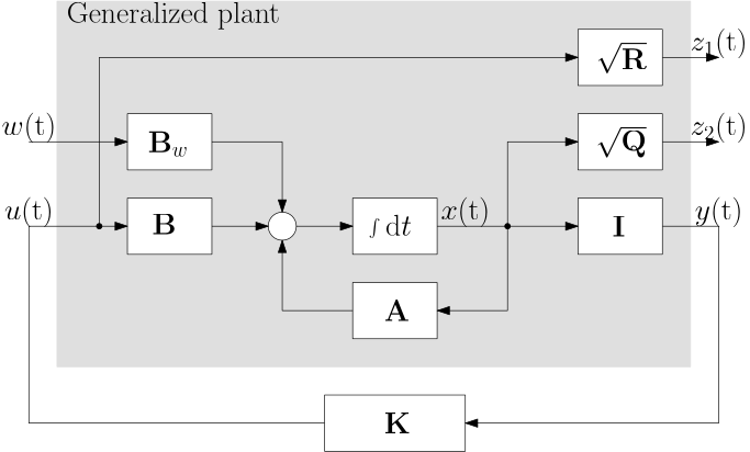
We now formulate the stochastic LQR problem as an input-output problem. Consider the block diagram in Fig. 3.
Figure 3: Stochastic LQR problem formulated as an interconnection of a (state) feedback controller and an artificial (also called generalized) plant
The grey block in Fig. 3 is our first instance of the so-called generalized plant. It has two inputs:
the white noise input \bm w(t),
the control input \bm u(t).
and two outputs:
the regulated output \bm z(t), here composed of two parts \bm z_1(t) and \bm z_2(t),
the measured output \bm y(t).
The optimal control problem is then formulated as
\operatorname*{minimize}_{\mathbf K} \mathbb E\left\{\begin{bmatrix}\bm z_1^\top(\infty)&\bm z_2^\top(\infty)\end{bmatrix}\begin{bmatrix}\bm z_1(\infty)\\ \bm z_2(\infty)\end{bmatrix}\right\}.
If this is not immediately visible, just use the fact that \bm z_1 = \sqrt{\mathbf R} \bm u and \bm z_2 = \sqrt{\mathbf Q} \bm x, and then \bm z_1^\top \bm z_1 = \bm u^\top \mathbf R \bm u and \bm z_2^\top \bm z_2 = \bm x^\top \mathbf Q \bm x.
The motivation for this reformulation will become clear in a moment.
\mathcal{H}_2 system norm
For a stable and strictly proper LTI system modelled by the (matrix) transfer function \mathbf G, the \mathcal{H}_2 norm is defined as \boxed{
\|\mathbf G\|_2 = \sqrt{\frac{1}{2\pi}\int_{-\infty}^\infty \text{Tr}\left[\mathbf G^\ast(j\omega)\mathbf G(j\omega)\right]\text{d}\omega},
}
where \text{Tr} is a trace of a matrix, that is, a sum of its diagonal elements.
Using Parseval’s theorem (relating inner products in time and frequency domains), we can rewrite the \mathcal{H}_2 norm as
\boxed{
\|\mathbf G\|_2 = \sqrt{\int_{0}^\infty \text{Tr}\left[\mathbf g^\top(t)\mathbf g(t)\right]\text{d}t},}
where \mathbf g(t) is the impulse response of the system with the transfer function \mathbf G(s). Clearly, it is equal to the \mathcal{L}_2 norm of the impulse response.
And why did we bother to introduce the \mathcal{H}_2 norm?
\mathcal{H}_2 norm as a gain of a system subject to a stationary white noise input
When presenting the following result, we restrict ourselves just to a single white noise input with the spectral density S_w. Equivalently, we can also consider a vector white noise with the spectral density matrix parameterized by a single parameter as in \mathbf S_w = S_w \mathbf I. The following result is useful:
It shows that the \mathcal H_2 system norm determines the root mean square (RMS) value of the steady-state output of the system subject to a white noise input. If the white noise input is of nonunit spectral density, the result is scaled by the square root of the spectral density of the input.
LQR viewed as \mathcal{H}_2-optimal control
Assembling the pieces together, we can now see that the reformulated LQR problem can be viewed as a special case of the \mathcal{H}_2 optimal control problem, for which the goal is to find a controller that minimizes the \mathcal{H}_2 norm of the closed-loop system.
Figure 4: Stochastic LQR as \mathcal{H}_2 optimal control problem (the controller is restricted to a matrix of gains)
This is certainly interesting, but once again – what is the point in all this? So far we have only reformulated our good old LQR problem in a new framework, but when it comes to solving the problem, we already know that the optimal solution can be found by solving the algebraic Riccati equation. We also know that the unique optimal controller is just a linear (proportional) state feedback controller.
Here comes the crucial fact: for a generalized plant (satisfying some minor technical conditions), not only the one in Fig. 3 corresponding to the LQR problem, there exists optimization solvers capable of finding a stabilizing feedback controller that minimizes the \mathcal H_2 norm of the closed-loop transfer function; see the section on software. Having been informed about this availability of solvers, how about modifying the generalized plant by changing the existing or adding some new blocks? Perhaps this could cover some new types of optimal control problem other than the LQR problem. For example, instead of the identity matrix \mathbf I in Fig. 3, we can use a general output matrix \mathbf C, which would allow us to use only a subset of the state variables for feedback control. Or we could add some first- or second-order filters right after the input \bm w, so that we can color the white noise input (to turn its flat spectral density into something frequency-dependent).
Indeed, this line of reasoning leads to a new broad family of optimal control problems, which is called \mathcal{H}_2 optimal control, diagrammed in Fig. 5. We emphasize that the controller is not restricted to a matrix of gains, but can also contain some dynamics, and as such can be modelled as a (matrix) transfer function.
Figure 5: General \mathcal{H}_2 optimal control problem (the controller can also contain some dynamics)
Although useful on its own, we get perhaps even better benefit from it by learning about the possibility to formulate an optimal control problem as a minimization of some system norm. We will encounter another system norm – the \mathcal{H}_\infty norm – in the next chapter, which will open up a whole new world of optimal control problems.
But before we do that, we are going to discuss another extension of the LQR problem – the popular LQG problem, which can also be formulated within the unified framework of \mathcal{H}_2 optimal control.