Components of DHA as inequalities

In this section, we use the general results from the previous section to show how the four components of the discrete hybrid automaton (DHA) can be formulated as linear inequalities and equations.

Finite state machine (FSM) using binary variables

For characterization of discrete states (both in discrete-event and hybrid systems), we used integer variables. But now, with anticipation of using numerical solvers, we will use binary variables. We encode the discrete state variable x_\mathrm{d} in binary. As a matter of fact, vector variables are needed here x_b \in \{0,1\}^{n_b}.

Similarly the discrete inputs u_b \in \{0,1\}^{m_b}.

The logic state equation then x_b(k+1) = f_b(x_b(k),u_b(k),\delta_e(k)).

Example 1 (Example)

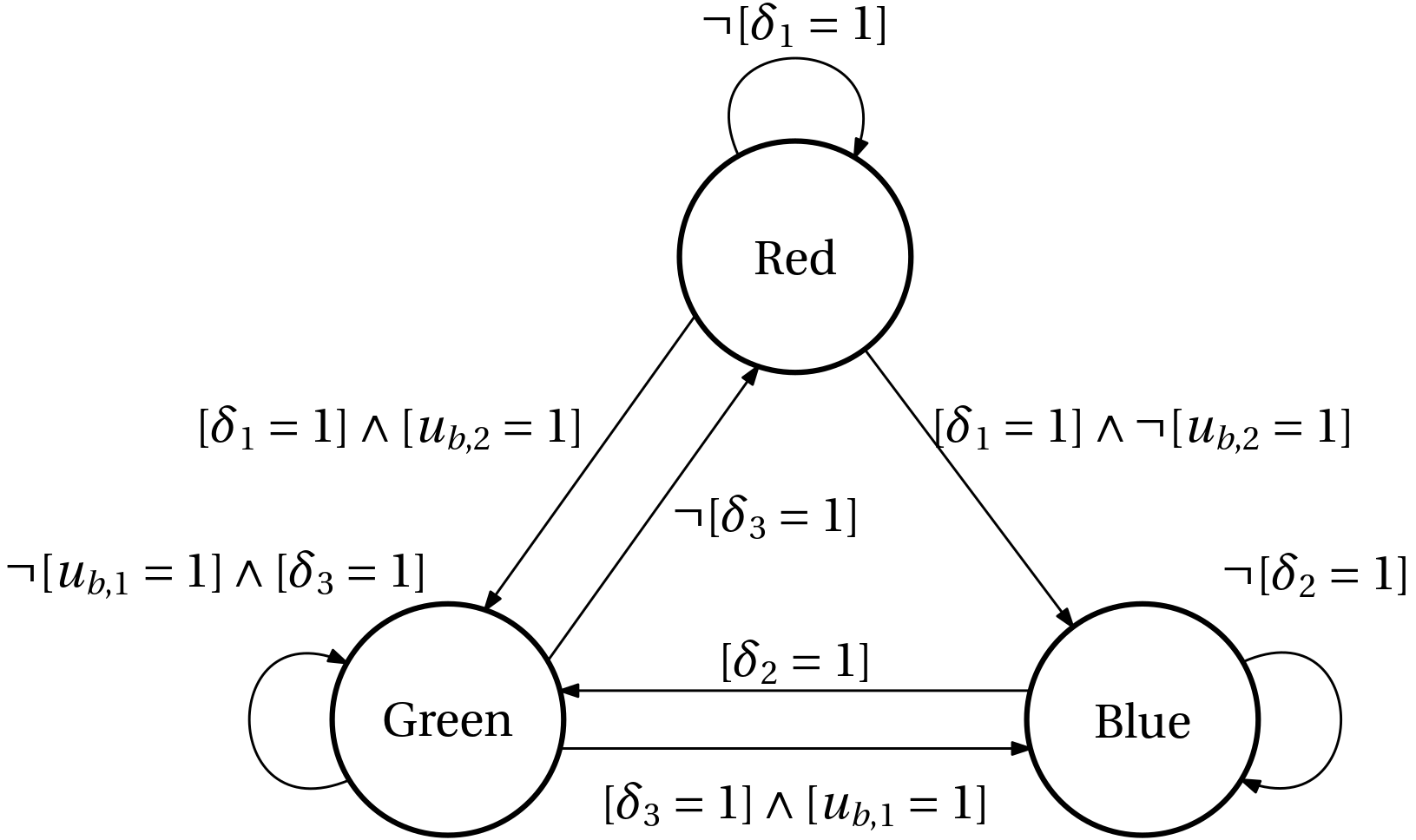
The state update/transition equation is \begin{aligned} x_d(k+1) = \begin{cases} \text{Red} & \text{if}\; ([x_d = \text{green}] \land \neg [\delta_3=1]) \lor ([x_d = \text{red}] \land \neg [\delta_3=1])\\ \text{Green} & \text{if} \; \ldots\\ \text{Blue} & \text{if} \; \ldots \end{cases} \end{aligned}

Binary encoding of the discrete states \text{Red}: x_b = \begin{bmatrix}0\\0 \end{bmatrix}, \; \text{Green}: x_b = \begin{bmatrix}0\\1 \end{bmatrix}, \; \text{Blue}: x_b = \begin{bmatrix}1\\0 \end{bmatrix}

Reformulating the state update equations for binary variables \begin{aligned} x_{b1} &= (\neg [x_{b1} = 1] \land \neg [x_{b2} = 1] \land [\delta_1=1] \land \neg[u_{b2}=1]) \\ &\quad \lor (\neg [x_{b1} = 1] \land [x_{b2} = 1] \land [\delta_3=1] \land [u_{b1}=1])\\ &\quad \lor ([x_{b1} = 1]\land [x_{b2} = 1] \land \neg [\delta_2=1])\\ x_{b2} &= \ldots \end{aligned}

Finally, simplify, convert to CNF.

Mixing logical and continuous through indicator variables

Now that we have learnt to encode purely logical expressions into inequalities, we consider the cases where logical and continuous variables are mixed. We aim at the same kind of encoding as before, that is, we want to formulate inequalities.

Logical implies continuous

We start by considering the implication X \rightarrow [f(x)\leq 0], where X is a Boolean variable and f(x) is a real-valued function of a real variable x. Upon represented the Boolean variable X with the binary variable \delta (called an indicator variable) we can write the implication as [\delta = 1] \rightarrow [f(x)\leq 0].

In order to construct an equivalent inequality, we introduce a real parameter M large enough such that when \delta=0 in f(x) \leq (1-\delta) M, there is no practical restriction on f. If \delta=1, the original inequality is trivially enforced.

Big-M technique

This is a popular trick and is known as the Big-M technique. It is not a trouble-free trick, though. It is important to avoid setting M unnecessarily too high. See the section Dealing with Big-M Constraints in Gurobi Reference Manual for some discussion of numerical issues.

Continuous implies logical

The other implication [f(x)\leq 0] \rightarrow X, with the Boolean variable X represented with a binary \delta as [f(x)\leq 0] \rightarrow [\delta = 1], can be written equivalently as \neg [\delta = 1] \rightarrow \neg [f(x)\leq 0], which can be further simplified to [\delta = 0] \rightarrow [f(x) > 0].

We now introduce m small enough such that that f(x) is practically unrestricted when \delta=1 in f(x) > m\delta, while f(x)>0 is trivially enforced when \delta=0.

For numerical reasons, we modify the strict equality to nonstrict inequality f(x) \geq \epsilon + (m-\epsilon)\delta, where \epsilon\approx 0 (for example, machine epsilon).

Equivalence between logical and continuous

Now we combine the previous two implications so that we can write the equivalence X \leftrightarrow [f(x)\leq 0],

represented through the indicator variable \delta as \boxed{ [\delta = 1] \leftrightarrow [f(x)\leq 0], }

as the two inequalities \boxed{ \begin{aligned} f(x) &\leq (1-\delta) M,\\ f(x) &\geq \epsilon + (m-\epsilon)\delta. \end{aligned}} \tag{1}

IF-THEN-ELSE rule as an inequality

We now consider the following IF-THEN-ELSE rule:

\mathrm{if} \; X, \; \mathrm{then} \; z = f(x,u), \; \text{else} \; z = 0.

It can be equivalently expressed as the product z = \delta\,f(x,u), where \delta is a binary indicator. This, in turn, can be written (finally using ?@eq-product-assignment) as \begin{aligned} z &\leq M\delta,\\ - z &\leq -m\delta,\\ z &\leq f(x,u) - m(1-\delta),\\ -z &\leq -f(x,u) + M(1-\delta). \end{aligned}

Scalar functions only

Beware that the above results are valid only for scalar functions f(), even if their arguments are possibly vectors.

Particularly useful from a computational viewpoint will be an affine function f(x,y) = ax + bu + e. We specialize the above inequalities to this case for later convenience. \boxed{ \begin{aligned} z &\leq M\delta,\\ - z &\leq -m\delta,\\ z &\leq ax + bu + e - m(1-\delta),\\ -z &\leq -(ax + bu + e) + M(1-\delta). \end{aligned}} \tag{2}

Another IF-THEN-ELSE rule

Another IF-THEN-ELSE rule (and here we already specialized it to affine functions) can also be useful:

\mathrm{if} \; X, \; \mathrm{then} \; z = a_1x + b_1u + e_1, \; \mathrm{else} \; z = a_2x + b_2u + e_2.

Using a binary indicator \delta, it can be expressed as z = {\color{blue}\delta}\,(a_1 x + b_1 u + e_1) + {\color{blue}(1-\delta)}(a_2 x + b_2 u + e_2), which can be rewritten as \boxed{ \begin{aligned} (m_2-M_1)\delta + z &\leq a_2 x + b_2 u + e_2,\\ (m_1-M_2)\delta - z &\leq -a_2 x - b_2 u - e_2,\\ (m_1-M_2)(1-\delta) + z &\leq a_1 x + b_1 u + e_1,\\ (m_2-M_1)(1-\delta) - z &\leq -a_1 x - b_1 u - e_1. \end{aligned}} \tag{3}

Generation of events by mixing logical and continuous variables in inequalities

Application of Eq. 1 to the ith event generator function h_i(x,u) leads to the following inequalities \boxed{ \begin{aligned} h_i(x_c(k), u_c(k)) &\leq M_i (1-\delta_{e,i}),\\ h_i(x_c(k), u_c(k)) &\geq \epsilon + (m_i-\epsilon) \delta_{e,i}. \end{aligned}} \tag{4}

Switched affine system

We are now ready to get rid of the IF-THEN(-ELSE) conditions in the definition of the switched affine system by reformulating it as inequalities. Namely, we compose the state variable in the next step as a sum of the auxiliary variables z_i: x_c(k+1) = \sum_{i=1}^s z_i(k), where z_1(k) = \begin{cases} a_1 x_c(k) + b_1 u_c(k) + f_1 & \text{if}\;i(k)=1,\\ 0 & \text{otherwise}, \end{cases} \quad \vdots z_s(k) = \begin{cases} a_s x_c(k) + b_s u_c(k) + f_s & \text{if}\;i(k)=s,\\ 0 & \text{otherwise}, \end{cases} and we rewrite it for each i\in \{1, 2, \ldots, s\} as \boxed{ \begin{aligned} z_i &\leq M_i\delta_i,\\ - z_i &\leq -m_i\delta_i,\\ z_i &\leq a_i x + b_i u + f_i - m_i(1-\delta_i),\\ -z_i &\leq -(a_i x + b_i u + f_i) + M_i(1-\delta_i). \end{aligned}} \tag{5}

All these results were derived just for scalar z and f()

With the formalism presented here, vector variables \bm z and correspondingly vector right-hand-side functions \mathbf f() must be handled but considering their individual scalar components z_1, \ldots, z_n and f_1(), \ldots, f_n(). Notational care must be exercised, note that the lower index in this remark has different meaning than that in Eq. 5.