Simulations of complementarity systems using time-stepping
One of the useful outcomes of the theory of complementarity systems is a new family of methods for numerical simulation of discontinuous systems. Here we will demonstrate the essence by introducing the method of time-stepping. And we do it by means of an example.
Example 1 (Simulation using time-stepping) Consider the following discontinuous dynamical system in \mathbb R^2:
\begin{aligned}
\dot x_1 &= -\operatorname{sign} x_1 + 2 \operatorname{sign} x_2\\
\dot x_2 &= -2\operatorname{sign} x_1 -\operatorname{sign} x_2.
\end{aligned}
Precompiling CairoMakie...
481.2 ms ✓ Graphics
685.0 ms ✓ FreeType
1317.4 ms ✓ Cairo
1494.7 ms ✓ FreeTypeAbstraction
3137.2 ms ✓ MathTeXEngine
27960.0 ms ✓ TiffImages
66238.1 ms ✓ Makie
24447.9 ms ✓ CairoMakie
8 dependencies successfully precompiled in 120 seconds. 267 already precompiled.
Figure 1: State portrait of the discontinuous system
One particular (vector) state trajectory obtained by some default ODE solver is in Fig. 2.
Figure 3: Trajectory of the discontinuous system in the state space
Note that for the default setting of absolute and relative tolerances, the adaptive-step ODE solver actually needed a huge number of steps:
Show the code
length(sol.t)
288594
This is indeed quite a lot. Can we do better?
In this particular example, we have the benefit of being able to analyze the solution analytically. In particular, we can ask: how fast does the solution approach the origin? We turn this into a question of how fast the distance from the origin decreases. With some anticipation we use the 1-norm \|\bm x\|_1 = |x_1| + |x_2| to the distance of the state from the origin. We then ask:
\frac{\mathrm d}{\mathrm dt}\|\bm x\|_1 = ?
We avoid the troubles with nonsmoothness of the absolute value by considering each quadrant separately. Let’s start in the first (upper right) quadrant, that is, x_1>0 and x_2>0, from which it follows that |x_1| = x_1, \;|x_2| = x_2, and therefore
\frac{\mathrm d}{\mathrm dt}\|\bm x\|_1 = \dot x_1 + \dot x_2 = 1 - 3 = -2.
The situation is identical in the other quadrants. We do not worry that the norm is undefined on the axes, because the trajectory obviously just crosses them.
The conclusion is that the trajectory will hit the origin in finite time (!): with, say, x_1(0) = 1 and x_2(0) = 1, the trajectory hits the origin at t=(|x_1(0)|+|x_2(0)|)/2 = 1. Surprisingly (or not), this will happen after an infinite number of revolutions around the origin…
We have seen above in Fig. 2 that a default solver for ODE can handle the situation in a decent way. But we have also seen that this was at the cost of a huge number of steps. To get some insight, we implement our own solver.
Forward Euler with fixed step size
We start with the simplest of all methods, the forward Euler method with a fixed step length. The computation of the next state is done just by the assignment
\begin{aligned}
{\color{blue}x_{1,k+1}} &= x_{1,k} + h (-\operatorname{sign} x_{1,k} + 2 \operatorname{sign} x_{2,k})\\
{\color{blue}x_{2,k+1}} &= x_{2,k} + h (-2\operatorname{sign} x_{1,k} - \operatorname{sign} x_{2,k}).
\end{aligned}
Blue color in our text is used to denote the unknown
We use the blue color here (and in the next few paragraphs) to highlight what is uknown.
Show the code
f(x) = [-sign(x[1]) +2*sign(x[2]), -2*sign(x[1]) -sign(x[2])]usingLinearAlgebraN =1000x₀ = [-1.0, 1.0] x = [x₀]tfinal =norm(x₀,1)/2tfinal =5.0h = tfinal/N t =range(0.0, step=h, stop=tfinal)for i=1:N xnext = x[i] +h*f(x[i]) push!(x,xnext)endX = [getindex.(x, i) for i in1:length(x[1])]Plots.plot(t,X,lw=3,label=false,xlabel="t",ylabel="x")
Figure 4: Solution trajectory for a discontinuous system obtained by the forward Euler method
Then number of steps is
Show the code
length(t)
1001
which is significantly less than before, but the solution is not perfect – notice the chattering. It could be reduced by using a smaller step size, but again, at the cost of a longer simulation time.
Backward Euler
As an alternative to the forward Euler method, we can use the backward Euler method. The computation of the next state is done by solving the nonlinear equations
\begin{aligned}
{\color{blue} x_{1,k+1}} &= x_{1,k} + h (-\operatorname{sign} {\color{blue}x_{1,k+1}} + 2 \operatorname{sign} {\color{blue}x_{2,k+1}})\\
{\color{blue} x_{2,k+1}} &= x_{2,k} + h (-2\operatorname{sign} {\color{blue}x_{1,k+1}} - \operatorname{sign} {\color{blue}x_{2,k+1}}).
\end{aligned}
The discontinuities on the right-hand sides constitute a challenge for solvers of nonlinear equations – recall that the Newton’s method requires the first derivatives (assembled into the Jacobian) or their approximation. Instead of this struggle, we can use the linear complementarity problem (LCP) formulation.
Formulation of the backward Euler using LCP
Instead solving the above nonlinear equations with discontinuities, we introduce new variables u_1 and u_2 as the outputs of the \operatorname{sign} functions:
\begin{aligned}
{\color{blue} x_{1,k+1}} &= x_{1,k} + h (-{\color{blue}u_{1}} + 2 {\color{blue}u_{2}})\\
{\color{blue} x_{2,k+1}} &= x_{2,k} + h (-2{\color{blue}u_{1}} - {\color{blue}u_{2}}).
\end{aligned}
But now we have to enforce the relationship between \bm u and \bm x_{k+1}. Recall the standard definition of the \operatorname{sign} function is
\operatorname{sign}(x) = \begin{cases}
1 & x>0\\
0 & x=0\\
-1 & x<0,
\end{cases}
but we change the definition to a set-valued function
\begin{cases}
\operatorname{sign}(x) = 1 & x>0\\
\operatorname{sign}(x) \in [-1,1] & x=0\\
\operatorname{sign}(x) = -1 & x<0.
\end{cases}
Accordingly, we set the relationship between \bm u and \bm x to
\begin{cases}
u_1 = 1 & x_1>0\\
u_1 \in [-1,1] & x_1=0\\
u_1 = -1 & x_1<0,
\end{cases}
and
\begin{cases}
u_2 = 1 & x_2>0\\
u_2 \in [-1,1] & x_2=0\\
u_2 = -1 & x_2<0.
\end{cases}
But these are mixed complementarity contraints we have defined previously! We can thus write the single step of the simulation algorithm as the MCP
\boxed{
\begin{aligned}
\begin{bmatrix}
{\color{blue} x_{1,k+1}}\\
{\color{blue} x_{2,k+1}}
\end{bmatrix}
&=
\begin{bmatrix}
x_{1,k}\\
x_{2,k}
\end{bmatrix} + h
\begin{bmatrix}
-1 & 2 \\
-2 & -1
\end{bmatrix}
\begin{bmatrix}
{\color{blue}u_{1}}\\
{\color{blue}u_{2}}
\end{bmatrix}\\
-1 &\leq {\color{blue} u_1} \leq 1 \quad \bot \quad -{\color{blue}x_{1,k+1}}\\
-1 &\leq {\color{blue} u_2} \leq 1 \quad \bot \quad -{\color{blue}x_{2,k+1}}.
\end{aligned}
}
\tag{1}
We now have enough to start implementing a solver for this system, provided we have an access to a solver the MCP (see the page dedicated to software for complementarity problems). But before we do it, we analyze the problem a bit deeper. In this particular small and simple case, it is still doable with just a pencil and paper.
9 possible combinations
There are now 9 possible combinations of the values of u_1 and u_2, each of them strictly inside their respective intervals, or at the either end. Let’s explore some combinations. We start with x_{1,k+1} = x_{2,k+1} = 0, while u_1 \in [-1,1] and u_2 \in [-1,1]:
How does the set of states from which the next state is zero look like? We isolate the vector \bm u from the equation and impose the constraints on it:
\begin{aligned}
-\begin{bmatrix}
-1 & 2 \\
-2 & -1
\end{bmatrix}^{-1}
\begin{bmatrix}
x_{1,k}\\
x_{2,k}
\end{bmatrix}
&= h
\begin{bmatrix}
{\color{blue}u_{1}}\\
{\color{blue}u_{2}}
\end{bmatrix}\\
-1 \leq {\color{blue} u_1} \leq 1, \quad -1 &\leq {\color{blue} u_2} \leq 1
\end{aligned}
We then get
\begin{bmatrix}
-h\\-h
\end{bmatrix}
\leq
\begin{bmatrix}
0.2 & 0.4 \\
-0.4 & 0.2
\end{bmatrix}
\begin{bmatrix}
x_{1,k}\\
x_{2,k}
\end{bmatrix}
\leq
\begin{bmatrix}
h\\ h
\end{bmatrix}
For h=0.2, the resulting set is a rotated square, as shown in Fig. 5.
Precompiling LazySets...
319.6 ms ✓ CodecBzip2
43324.4 ms ✓ MathOptInterface
3618.6 ms ✓ GLPK
10483.1 ms ✓ JuMP
6316.9 ms ✓ LazySets
5 dependencies successfully precompiled in 61 seconds. 82 already precompiled.
Precompiling OptimMOIExt...
1274.8 ms ✓ Optim → OptimMOIExt
1 dependency successfully precompiled in 2 seconds. 92 already precompiled.
Figure 5: The set of states from which the next state is zero (the origin)
Indeed, if the current state is in this rotated square, then the next state will be zero. No more infite spiralling around the origin! No more chattering! Perfect zero.
Another combination
We now consider u_1 = 1, u_2 = 1, which we substitute into Eq. 1:
\begin{aligned}
\begin{bmatrix}
{\color{blue} x_{1,k+1}}\\
{\color{blue} x_{2,k+1}}
\end{bmatrix}
&=
\begin{bmatrix}
x_{1,k}\\
x_{2,k}
\end{bmatrix} + h
\begin{bmatrix}
-1 & 2 \\
-2 & -1
\end{bmatrix}
\begin{bmatrix}
{1}\\
{1}
\end{bmatrix}\\
\color{blue}x_{1,k+1} &\geq 0\\
\color{blue}x_{2,k+1} &\geq 0,
\end{aligned}
which can be reformatted to
\begin{bmatrix}
x_{1,k}\\
x_{2,k}
\end{bmatrix} + h
\begin{bmatrix}
-1 & 2 \\
-2 & -1
\end{bmatrix}
\begin{bmatrix}
1\\
1
\end{bmatrix}\geq \bm 0,
and further to
\begin{bmatrix}
x_{1,k}\\
x_{2,k}
\end{bmatrix}
\geq h
\begin{bmatrix}
-1\\
3
\end{bmatrix}.
The set of states for which the next state is such that both its state variables are positive (hence u_1 = 1, u_2 = 1) is shown in Fig. 6.
Figure 7: The nine regions of the state space for the spiralling system
Solutions using a MCP solver
Now that we have got some insight into the algorithm, we can implement it by wrapping a for-loop around the MCP solver.
Show the code
M = [-12; -2-1]h =2e-1tfinal =2.0N = tfinal/hx0 = [-1.0, 1.0]x = [x0]usingJuMPusingPATHSolverfor i =1:N model =Model(PATHSolver.Optimizer)set_optimizer_attribute(model, "output", "no")set_silent(model)@variable(model, -1<= u[1:2] <=1)@constraint(model, -h*M * u - x[end] ⟂ u)optimize!(model)push!(x, x[end]+h*M*value.(u))end
Precompiling PATHSolver...
1732.0 ms ✓ PATHSolver
1 dependency successfully precompiled in 2 seconds. 65 already precompiled.
The code is admittedly unoptimized (for example, it is not wise to start building the optimization model from the scratch in every iteration), but it was our intention to keep it simple to be read conveniently.
The code outcome can be plotted as in Fig. 8. A solution obtained by a classical (default) ODE solver with default setting is plotted for comparison.
Show the code
t =range(0.0, step=h, stop=tfinal)X = [getindex.(x, i) for i in1:length(x[1])]usingPlotsPlots.plot(Ha, aspect_ratio=:equal,xlabel="x₁",ylabel="x₂",label=false,xlims=(-1.5,1.5),ylims=(-1.5,1.5))Plots.plot!(Hb)Plots.plot!(Hc)Plots.plot!(Hd)Plots.plot!(He)Plots.plot!(X[1],X[2],xlabel="x₁",ylabel="x₂",label="Time-stepping",aspect_ratio=:equal,lw=3,markershape=:circle)Plots.plot!(sol[1,:],sol[2,:],label=false,lw=3)
Figure 8: Solution trajectory for a discontinuous system obtained by the MCP solver
It is worth emphasizing that once the solution trajectory hits the blue square, it is just one step from the origin. And once the solution trajectory reaches the origin, it stays there forever, no more spiralling, no more chattering.
Apparently, the chosen step length was too large. If we reduce it, the resulting trajectory resembles the one obtained by a default ODE solver, as shown in Fig. 9.
Show the code
M = [-12; -2-1]h =1e-2tfinal =2.0N = tfinal/hx0 = [-1.0, 1.0]x = [x0]usingJuMPusingPATHSolverfor i =1:N model =Model(PATHSolver.Optimizer)set_optimizer_attribute(model, "output", "no")set_silent(model)@variable(model, -1<= u[1:2] <=1)@constraint(model, -h*M * u - x[end] ⟂ u)optimize!(model)push!(x, x[end]+h*M*value.(u))endt =range(0.0, step=h, stop=tfinal)X = [getindex.(x, i) for i in1:length(x[1])]Plots.plot(X[1],X[2],xlabel="x₁",ylabel="x₂",label="Time-stepping",aspect_ratio=:equal,lw=3,markershape=:circle)Plots.plot!(sol[1,:],sol[2,:],lw=3,label="Default ODE solver with adaptive step")
Figure 9: Solution trajectory for a discontinuous system obtained by the MCP solver with a smaller step size
And yet the total number of steps is still much smaller:
Show the code
length(t)
201
Example 2 (Time-stepping for a mechanical system with a hard stop) Let’s now apply the time-stepping method for a mechanical system with a hard stop as described in the Example 2 in the section on complementarity systems. We start by formulating the semi-explicit Euler scheme
\begin{aligned}
\bm x_{k+1} &= \bm x_k + h \bm v_{k+1}\\
\bm v_{k+1} &= \bm v_k + h \mathbf A \bm x_{k} + h \mathbf B \bm u_k,
\end{aligned}
where
\mathbf A = \begin{bmatrix} -\frac{k_1+k2}{m_1} & \frac{k_2}{m_1}\\ \frac{k_2}{m_2} & -\frac{k_2}{m_2} \end{bmatrix}, \quad
\mathbf B = \begin{bmatrix} \frac{1}{m_1} & -\frac{1}{m_1}\\ 0 & \frac{1}{m_2} \end{bmatrix}.
Substituting from the second to the first equation, we get
{\color{blue}\bm x_{k+1}} = \bm x_k + h \bm v_k + h^2 \mathbf A \bm x_k + h^2 \mathbf B {\color{blue}\bm u_k},
in which we again highlight the unknown terms by blue color for convenience. These two vector unknowns must satisfy the following complementarity condition
0 \leq x_{1,k+1} \perp u_{1,k} \geq 0,
and
0 \leq (x_{2,k+1} - x_{1,k+1}) \perp u_{2,k} \geq 0.
This can be written compactly as
\bm 0 \leq \mathbf C \bm x_{k+1} \perp \bm u_{k} \geq 0,
where \mathbf C is known from the previous section as
\mathbf C = \begin{bmatrix}1 & 0\\ -1 & 1\end{bmatrix}.
The constraint can be expanded into
\bm 0 \leq \mathbf C\left(\bm x_k + h \bm v_k + h^2 \mathbf A \bm x_k + h^2 \mathbf B {\color{blue}\bm u_k}\right) \perp \bm u_{k} \geq 0,
which is an LCP problem with \bm q = \mathbf C\left(\bm x_k + h \bm v_k + h^2 \mathbf A \bm x_k\right) and \mathbf M = h^2 \mathbf C \mathbf B.
An implementation of the time-stepping for this system is shown below.
Note, once again, the amazingly small number of steps
Show the code
length(t)
101
while the shape of the trajectory is already quite accurate (you can try reducing the step lenght by yourself)and whatever chattering is absent in the solution.
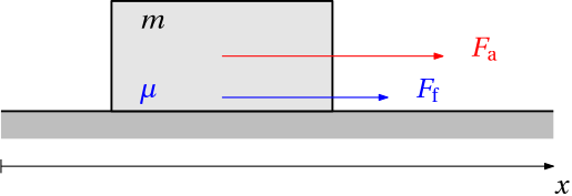
Example 3 (Time stepping for a mechanical system with Coulomb friction modelled as complementarity constraints) We consider an object of mass m moving on a horizontal surface. The object is subject to an applied force F_\mathrm{a} and a friction force F_\mathrm{f}, both oriented in the positive direction of position and velocity, as in Fig. 10.
Figure 10: Coulomb friction to be modelled using complementarity constraints
The friction force is modelled as a Coulomb friction model
F_\mathrm{f}(t) = -m g \mu\, \mathrm{sgn}(v(t)),
where \mu is a coefficient that relates the frictional force to the normal force mg.
The motion equations are
\begin{aligned}
\dot x(t) &= v(t)\\
\dot v(t) &= \frac{1}{m}(F_\mathrm{a}(t) + F_\mathrm{f}(t)).
\end{aligned}
We now express the friction force as a difference of two nonnegative variables
F_\mathrm{f}(t) = F^+_\mathrm{f}(t) - F^-_\mathrm{f}(t),\quad F^+_\mathrm{f}(t), \,F^-_\mathrm{f}(t) \geq 0.
And we also introduce another auxiliary variable \nu(t) that is just the absolute value of the velocity
\nu(t) = |v(t)|.
With the three new variables we formulate the Coulomb friction model as
\begin{aligned}
0 \leq v + \nu &\perp F^+_\mathrm{f} \geq 0,\\
0 \leq -v + \nu &\perp F^-_\mathrm{f} \geq 0, \\
0 \leq \mu m g - F^+_\mathrm{f} - F^-_\mathrm{f} &\perp \nu \geq 0.
\end{aligned}
If F^-_\mathrm{f} > 0, that is, if the friction force is negative, the second complementarity constraint implies that the velocity is equal to its absolute value, in other words, it is nonnegative, the object moves to the right (or stays still). If the velocity is positive, the first constraint implies that F^+_\mathrm{f} = 0, and the third constraint then implies that F^-_\mathrm{f} = mg\mu. Feel free to explore other cases.
We now proceed to implement the time-stepping method for this system. Once again, we use the semi-explicit Euler scheme
\begin{aligned}
x_{k+1} &= x_k + h v_{k+1},\\
v_{k+1} &= v_k + \frac{h}{m} (F^+_{\mathrm{f},k} - F^-_{\mathrm{f},k}),
\end{aligned}
where the velocity is subject to the complementarity constraints
\begin{aligned}
0 \leq v_{k+1} + \nu_{k+1} &\perp F^+_{\mathrm{f},k} \geq 0,\\
0 \leq -v_{k+1} + \nu_{k+1} &\perp F^-_{\mathrm{f},k} \geq 0, \\
0 \leq \mu m g - F^+_{\mathrm{f},k} - F^-_{\mathrm{f},k} &\perp \nu_{k+1} \geq 0,
\end{aligned}
into which we substitute for v_{k+1}\boxed{
\begin{aligned}
0 \leq v_k + \frac{h}{m} ({\color{blue}F^+_{\mathrm{f},k}} - {\color{blue}F^-_{\mathrm{f},k}}) + {\color{blue}\nu_{k+1}}\, &\perp\, {\color{blue}F^+_{\mathrm{f},k}} \geq 0,\\
0 \leq -\left(v_k + \frac{h}{m} ({\color{blue}F^+_{\mathrm{f},k}} - {\color{blue}F^-_{\mathrm{f},k}})\right) + {\color{blue}\nu_{k+1}}\, &\perp\, {\color{blue}F^-_{\mathrm{f},k}} \geq 0, \\
0 \leq \mu m g - {\color{blue}F^+_{\mathrm{f},k}} - {\color{blue}F^-_{\mathrm{f},k}} \,&\perp\, {\color{blue}\nu_{k+1}} \geq 0,
\end{aligned}
}
in which we highlighted the unknowns by blue color for convenience.
Once again, we can see that the method correctly simulates the system coming to a complete stop due to friction.
Important
While concluding this section about time-stepping methods, we have to emphasize that this was really just an introduction. But the essence of using complementarity concepts in numerical simulation is perhaps a bit clearer now.