Complementarity systems
Linear complementarity system (LCS)
Having introduced the complementarity constraints and optimization problems with these constraints, we can now show how these constraints can be used to model a certain class of dynamical systems – complementarity dynamical systems. We start with linear ones, namely, linear complementarity systems (LCS). These are also called in the literature as Linear dynamical complementarity problems (LDCP).
Linear complementarity system is modelled by \boxed{ \begin{aligned} \dot{\bm x}(t) &= \mathbf A \bm x(t) + \mathbf B\bm u(t)\\ \bm y(t) &= \mathbf C \bm x(t) + \mathbf D\bm u(t)\\ \mathbf 0&\leq \bm u(t) \perp \bm y(t) \geq \mathbf 0. \end{aligned}} \tag{1}
Example 1 (Electrical circuit with a diode as an LCS)
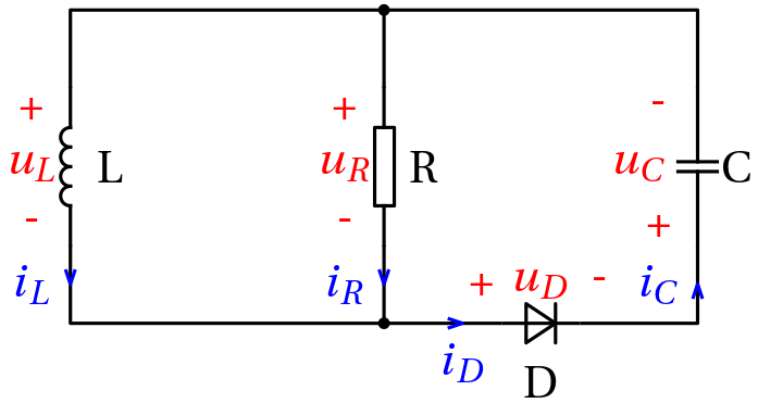
Note the upside-down orientation of the voltage and the current for the capacitor – we wanted the diode current identical to the capacitor current.
Following the charge formalism within Lagrangian modelling, we can choose the generalized coordinates as \bm q = \begin{bmatrix} q_L \\ q_C \end{bmatrix}.
That this is indeed a sufficient number is obvious, but we can also check the classical formula B-N+1 = 4-3+1 = 2. But we can also choose the state variables as \bm x = \begin{bmatrix} i_L\\ q_c \end{bmatrix}.
The resulting state equations are \begin{aligned} i_L' &= -\frac{1}{LC}q_C - \frac{1}{L}u_D\\ q_C' &= i_L - \frac{1}{RC} q_C - \frac{1}{R} u_D. \end{aligned}
The idealized volt-ampere characteristics of the diode is
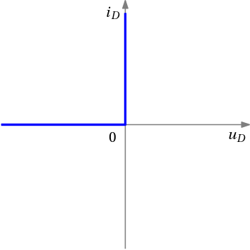
Flipping the axes to get the current as the horizontal axis, we get
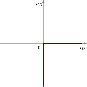
Finally, after introducing an auxiliary variable (the reverse voltage of the diode) \bar u_D = -u_D , we get the desired dependence
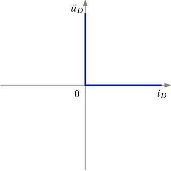
which can be modelled as a complementarity constraint
0\leq i_D \perp \bar u_D \geq 0.
Now, upon replacing the diode voltage with its reverse \bar u_D while using i_D=i_C, we get \begin{aligned} i_L' &= -\frac{1}{LC}q_C + \frac{1}{L} \bar u_D\\ q_C' &= i_L - \frac{1}{RC} q_C + \frac{1}{R} \bar u_D\\ 0&\leq q_C' \perp \bar u_D \geq 0. \end{aligned}
We are not there yet – there is a derivative in the complementarity constraint. But just substitute for it:
\begin{aligned}
i_L' &= -\frac{1}{LC}q_C + \frac{1}{L} \bar u_D\\
q_C' &= i_L - \frac{1}{RC} q_C + \frac{1}{R} \bar u_D\\
0&\leq i_L - \frac{1}{RC} q_C + \frac{1}{R} \bar u_D \perp \bar u_D \geq 0,
\end{aligned}
and voila, we finally got the LCS description. We can also reformat it into the matrix-vector form
\begin{aligned}
\begin{bmatrix}
i_L' \\ q_C'
\end{bmatrix} &=
\begin{bmatrix}
0 &-\frac{1}{LC}\\
1 & - \frac{1}{RC}
\end{bmatrix}
\begin{bmatrix}
i_L \\ q_C
\end{bmatrix} +
\begin{bmatrix}
\frac{1}{L}\\
\frac{1}{R}
\end{bmatrix}
\bar u_D\\
0 &\leq \left(\begin{bmatrix}
1 & - \frac{1}{RC}
\end{bmatrix}
\begin{bmatrix}
i_L \\ q_C
\end{bmatrix} +
\begin{bmatrix}
\frac{1}{L}\\
\frac{1}{R}
\end{bmatrix}
\bar u_D\right ) \bot \bar u_D \geq 0.
\end{aligned}
Example 2 (Mass-spring system with a hard stop as a linear complementarity system) Two carts moving horitontally (left or right) are interconnected through a spring. The left cart is also interconnected with the wall through a another spring. Furthemore, the motion of the left cart is constrained in that there is a hard stop that prevents the cart from moving further to the left. Another natural constraint is that the right cart cannot get to the left of the other vehicle. The setup is shown in Fig. 1.

The variables x_1 and x_2 give deviations of the two carts from their equilibrium positions. As we are considering negligible sizes of the two carts, the equilibrium position for both is 0. The derivatives of the two positions are also introduced as state variables x_3 and x_4, respectively.
The hard stop is located at the equilibrium position of the left cart.
The input u_1 corresponds to the reaction force of the hard stop applied to the left cart. Another input is u_2 that corresponds to the force exerted by the left cart onto the right cart.
The state equations are \begin{aligned} \dot x_1(t) &= x_3,\\ \dot x_2(t) &= x_4,\\ \dot x_3(t) &= -\frac{k_1+k_2}{m_1}x_1(t) + \frac{k_2}{m_1}x_2(t) + \frac{1}{m_1}u_1(t) - \frac{1}{m_1}u_2(t),\\ \dot x_4(t) &= \frac{k_2}{m_2}x_1(t) - \frac{k_2}{m_2} x_2(t) + \frac{1}{m_2}u_2(t). \end{aligned}
The presence of the hard stop can be modelled as an inequality constraint on the state x_1(t) \geq 0.
Similarly, the fact that the right cart cannot get to the left of the left cart can be expressed as x_2(t) - x_1(t) \geq 0.
This motivates us to define two output variables as \begin{aligned} y_1(t) &= x_1(t),\\ y_2(t) &= x_2(t)-x_1(t). \end{aligned}
Now, the reaction force u_1 exerted by the hard stop onto the left cart can only be nonnegative
u_1(t) \geq 0,
and it is positive if and only if the left cart hits the hard stop
y_1(t) u_1(t) = 0.
The condition can be written compactly as 0\leq y_1(t) \perp u_1(t) \geq 0.
Similarly for the force u_2 exerted by the left cart onto the right cart 0\leq y_2(t) \perp u_2(t) \geq 0.
For convenience, we now give a full model in the matrix-vector form. \begin{aligned} \begin{bmatrix} \dot x_1\\ \dot x_2\\ \dot x_3\\ \dot x_4 \end{bmatrix} &= \begin{bmatrix} 0 & 0 & 1 & 0\\ 0 & 0 & 0 & 1\\ {\color{blue}-\frac{k_1+k_2}{m_1}} & {\color{blue}\frac{k_2}{m_1}} & 0 & 0\\ {\color{blue}\frac{k_2}{m_2}} & {\color{blue}-\frac{k_2}{m_2}} & 0 & 0 \end{bmatrix} \begin{bmatrix} x_1\\ x_2\\ x_3\\ x_4 \end{bmatrix} + \begin{bmatrix} 0 & 0\\ 0 & 0\\ {\color{blue}\frac{1}{m_1}} & {\color{blue}-\frac{1}{m_1}}\\ {\color{blue}0} & {\color{blue}\frac{1}{m_2}}\end{bmatrix} \begin{bmatrix} u_1\\u_2\end{bmatrix},\\ \begin{bmatrix} y_1 \\ y_2 \end{bmatrix} &= \begin{bmatrix} {\color{blue}1} & {\color{blue}0} & 0 & 0\\ {\color{blue}-1} & {\color{blue}1} & 0 & 0\end{bmatrix} \begin{bmatrix} x_1\\ x_2\\ x_3\\ x_4 \end{bmatrix},\\ \mathbf 0 &\leq \bm y \perp \bm u \geq \mathbf 0. \end{aligned} \tag{2}
Note that we highlighted in blue three submatrices that will come in handy in the next section.
Complementarity system as a feedback interconnection
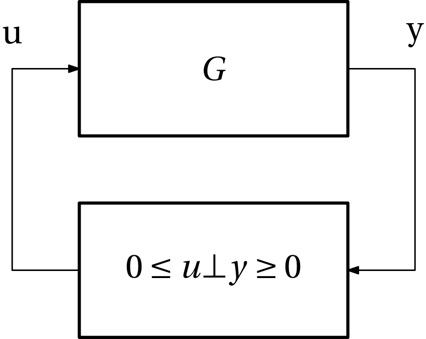
A complementarity system Eq. 1 can be seen as a feedback interconnection of a linear system and a complementarity constraint.
Complementarity systems vs PWA and max-plus linear systems
Consider the feedback interconnection of a dynamical system and the max(y,u) function in the feedback loop as in Fig. 2.
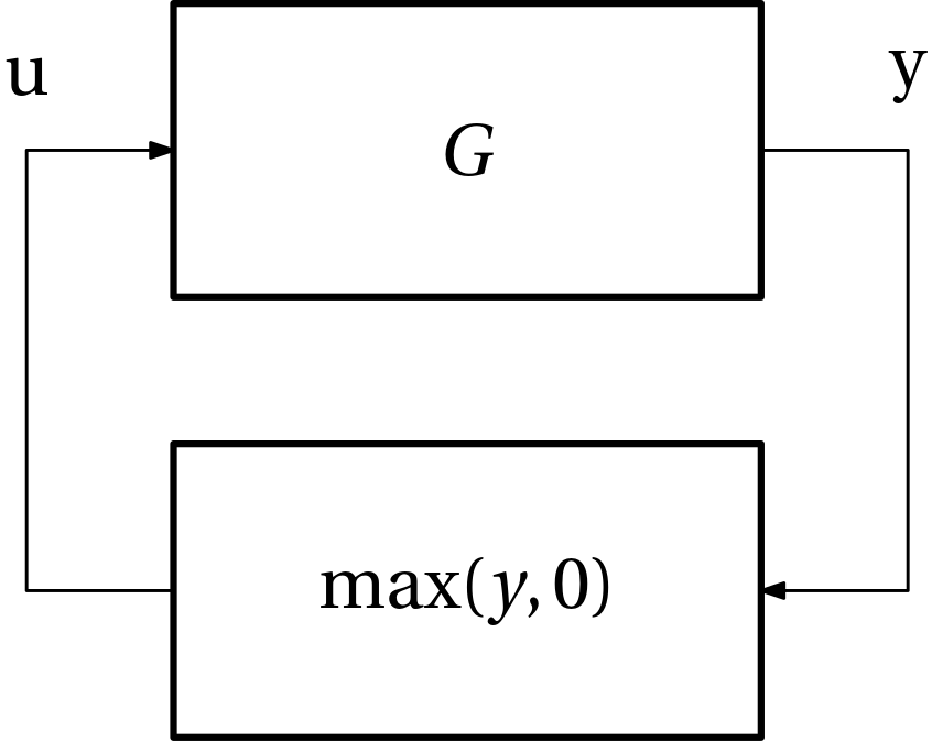
We now express the original y as a difference of two nonnegative variable satisfying the complementarity constraint y = y^+ - y^-,\quad 0 \leq y^+ \bot y^- \geq 0.
The motivation for this was that with the new variables y^+ and y^-, the max function can be expressed as \max(y,0) = \max(y^+ - y^-, 0) = y^+.
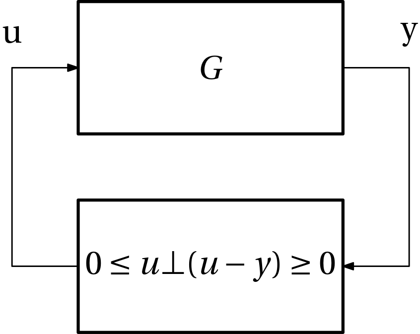
Now, set y^+ = u and then y = u - y^-, from which y^- = u - y and therefore the original feedback interconnection can be rewritten as
More complicated PWA functions in feedback
The function \max(y,0) that we have just considered is a very simple piecewise affine (PWA) function. But we can consider more complicated PWA functions. Only a little bit complicated PWA function is in Fig. 3.
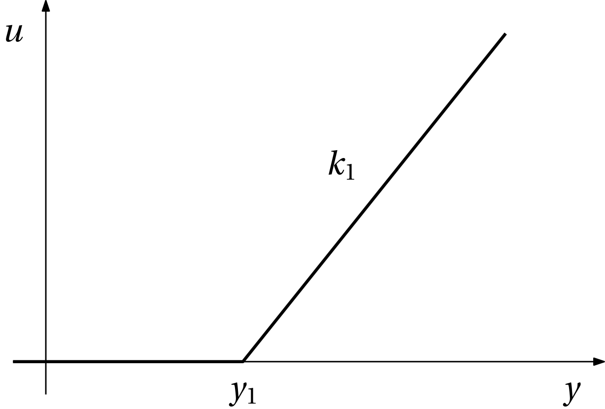
The function is defined by shifting and scaling the original \max(y,0) function: u(y) = k_1 \max(y-y_1,0) = \max(k_1(y-y_1),0).
We can now enforce complementarity based on this function in the feedback loop, see Fig. 4.
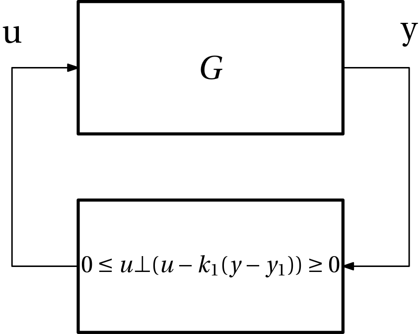
This procedure can be extended towards PWA functions composed of several segments, see Fig. 5.
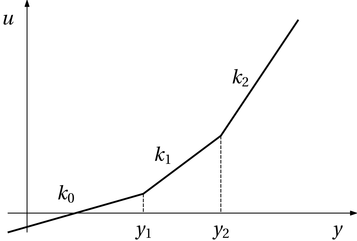
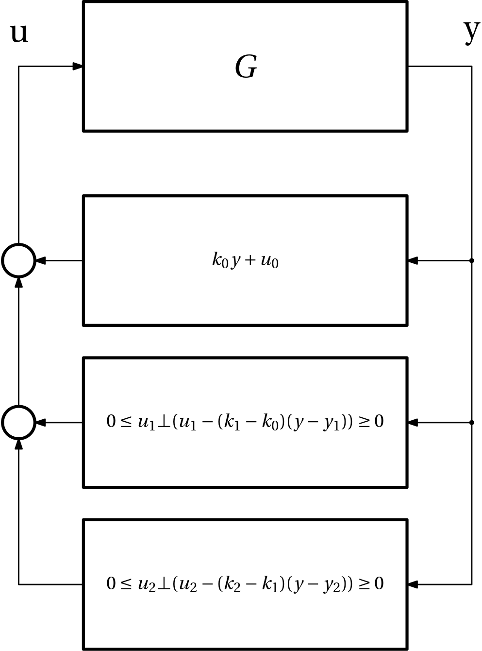
The function is defined as \begin{aligned} u(y) &= k_0 y + u_0 + (k_1-k_0) \max(y-y_1,0) \\ &\qquad + (k_2-k_1) \max(y-y_2,0)\\ &= k_0 y + u_0 + \underbrace{\max((k_1-k_0)(y-y_1),0)}_{u_1}\\ &\qquad + \underbrace{\max((k_2-k_1)(y-y_2),0)}_{u_2} \end{aligned} and the feedback interconnection now contain several parallel paths with complementarity constraints as in Fig. 6
