Hybrid automata
Well, here we are at last. After these three introductory topics on discrete-event systems, we’ll finally get into hybrid systems.
There are two frameworks for modelling hybrid systems:
- hybrid automaton, and
- hybrid (state) equations.
Here we start with the former and save the latter for the next chapter/week.
First we consider an autonomous (=no external/control inputs) hybrid automaton – it is a tuple of sets and (set) mappings \boxed{ \mathcal{H} = \{\mathcal Q, \mathcal Q_0, \mathcal X, \mathcal X_0, f, \mathcal I, \mathcal E, \mathcal G, \mathcal R\},} where
\mathcal Q is a set of discrete states (also called modes or operating modes or locations).
- Examples:
- \mathcal Q = \{\text{on}, \text{off}\},
- \mathcal Q = \{\text{working}, \text{broken},\text{in repair}\},
- \mathcal Q = \{\text{gear}\,1, \ldots, \text{gear}\,5\} .
- It can be characterized either by
- by enumeration like above, or
- using a state variable q(t) attaining discrete values. The variable can also be a vector one, possibly a binary vector state variable encoding an integer scalar state variable.
- Examples:
\mathcal Q_0\subseteq \mathcal Q is a set of initial discrete states.
- It can contain only a single element.
- Example: \mathcal Q_0 = \{\text{off}\}.
- But if it contains more than one element, it can be used to represent uncertainty in the initial state.
- It can contain only a single element.
\mathcal X\subseteq \mathbb R^n is a set of continuous states.
- Rather than by enumeration as in the case of discrete state, it is characterized by real-valued state variables x, oftentimes vector ones \bm x. Often they are denoted \bm x(t) to emphasize the evolution in time.
\mathcal X_0\subseteq \mathcal X is a set of initial continuous states.
- A set of values of the (vector) state variable at the initial time.
- Often just a single initial state \mathcal X_0=\{x_0\}, but it can be useful to set ranges of the values of individual state variables to account for uncertainty.
f:\mathcal{Q}\times \mathcal X \rightarrow \mathbb R^n is a vector field parameterized by the location
Often the dependence on the location q expressed as f_q(x) rather than the more symmetric f(q,x).
This defines a state equation parameterized by the location: \dot{x}(t) = f_q(x(t)).
It is also possible to consider a set-valued map, replacing f with \mathcal F: \mathcal{Q}\times \mathcal X \rightarrow 2^{\mathbb R^n}, which leads to the differential inclusion \dot x \in \mathcal F_q(x).
\mathcal I: \mathcal Q \rightarrow 2^\mathcal{X} gives a (location) invariant. It is also called a domain (of the location). The latter term is perhaps more appropriate because the term invariant is already too much overloaded in the context of dynamical systems.
- It is parameterized by the location.
- It is a subset of the continuous-valued state space \mathcal I(q) \subseteq \mathbb R^n.
- It is a set of values that the state variables are allowed to attain while staying in the given location; if the state of the systems evolves towards the boundary of this set with a tendency to leave it, the system must be ready to leave that location by transitioning to another location.
Strictly speaking, \mathcal{I} is a mapping and not a set. Only the mapping evaluated at a given location q, that is, \mathcal{I}(q), is a set.
\mathcal E\subseteq \mathcal Q \times \mathcal Q is a set of transitions.
- It is a set of the edges of the graph.
- Example: \mathcal E = \{(\text{off},\text{on}),(\text{on},\text{off})\}, that is, a two-component set.
\mathcal G: \mathcal E \rightarrow 2^\mathcal{X} gives a guard set.
- It is associated with a given transition. In particular, \mathcal G(q_i,q_j) is the guard set for the transition (q_i,q_j)\in\mathcal E.
- The guard condition for the given transition is satisfied if x\in \mathcal G(q_i,q_j).
- If the guard condition is satisfied, the transition is enabled – it may be executed. But it does not have to.
- The enabled transition must be executed when the state x leaves the invariant set of the original location.
- It is associated with a given transition. In particular, \mathcal G(q_i,q_j) is the guard set for the transition (q_i,q_j)\in\mathcal E.
\mathcal R: \mathcal E \times \mathcal X\rightarrow 2^{\mathcal X} is a reset map.
- For a given transition from one location to another, it resets the continuous-valued state x to a new value within some subset.
- Often the map is single-valued, r: \mathcal E \times \mathcal X\rightarrow \mathcal X (multivalued-ness can be used to model uncertainty).
- We also say that the state experiences a jump.
- The state after the jump (associated with the given transition) is reset according to x^+ = r(q_i,q_j, x), or x^+ \in \mathcal R(q_i,q_j, x) in the multivalued case.
- If no resetting of the continuous-valued state takes place, the reset map is defined just as the identity operator with respect to x , that is, r(q_i,q_j, x) = x.
Example 1 (Thermostat – the hello world example of a hybrid automaton) The thermostat is a device that turns some heater on or off (or sets some valve open or closed) based on the sensed temperature. The goal is to keep the temperature around, say, 18^\circ C.
Naturally, the discrete states (modes, locations) are on and off. Initially, the heater is off. We can identify the first two components of the hybrid automaton: \mathcal Q = \{\text{on}, \text{off}\}, \quad \mathcal Q_0 = \{\text{off}\}
The only continuous state variable is the temperature. The initial temperature is not quite certain, say, it is known to be in the interval [5,10]. Two more components of the hybrid automaton follow: \mathcal X = \mathbb R, \quad \mathcal X_0 = \{x:x\in \mathcal X, 5\leq x\leq 10\}
In the two modes on and off, the evolution of the temperature can be modelled by two different ODEs. Either from first-principles modelling or from system identification (or preferrably from the combination of the two) we get the two differential equations, say:
f_\text{off}(x) = -0.1x,\quad f_\text{on}(x) = -0.1x + 5,
which gives another component for the hybrid automaton.
The control logic of the thermostat is captured by the \mathcal I and \mathcal G components of the hybrid automaton. Let’s determine them now. Obviously, if we just set 18 as the threshold, the heater would be switching on and off all the time. We need to introduce some hysteresis. Say, keeping the temperature within the interval (18 \pm 2)^\circ C is acceptable. \mathcal I(\text{off}) = \{x\mid x> 16\},\quad \mathcal I(\text{on}) = \{x\mid x< 20\},
\mathcal G(\text{off},\text{on}) = \{x\mid x\leq 17\},\; \mathcal G(\text{on},\text{off}) = \{x\mid x\geq 19\}.
Finally, \mathcal R (or r) is not specified as the x variable (the temperature) doesn’t jump. Well, it is specified implicitly as an identity mapping r(x)=x.
The graphical representation of the thermostat hybrid automaton is shown in Fig. 1.

Is this model deterministic? There are actually two reasons why it is not:
- If we regard the characterization of the initial state (the temperature in this case) as a part of the model, which is the convention that we adhere to in our course, the model is nondeterministic.
- Since the invariant for a given mode and the guard set for the only transition to the other model overlap, the response of the system is not uniquely determined. Consider the case when the system is in the
offmode and the temperature is 16.5. The system can either stay in theoffmode or switch to theonmode.
Hybrid automaton with external events and control inputs
We now extend the hybrid automaton with two new components:
- a set \mathcal{A} of (external) events (also actions or symbols),
- a set \mathcal{U} external continuous-valued inputs (control inputs or disturbances).
\boxed{ \mathcal{H} = \{\mathcal Q, \mathcal Q_0, \mathcal X, \mathcal X_0, \mathcal I, \mathcal A, \mathcal U, f, \mathcal E, \mathcal G, \mathcal R\} ,} where
\mathcal A = \{a_1,a_2,\ldots, a_s\} is a set of events
- The role identical as in a (finite) state automaton: an external event triggers an (enabled) transition from the current discrete state (mode, location) to another.
- Unlike in pure discrete-event systems, here they are considered within a model that does recognize passing of time – each action must be “time-stamped”.
- In simulations such timed event can be represented by an edge in the signal. In this regard, it might be tempting not to introduce it as a seperate entity, but it is useful to do so.
\mathcal U\in\mathbb R^m is a set of continuous-valued inputs
- Real-valued functions of time.
- Control inputs, disturbances, references, noises. In applications it will certainly be useful to distinghuish these roles, but here we keep just a single type of such an external variable, we do not have to distinguish.
Some modifications needed
Upon introduction of these two types of external inputs we must modify the components of the definition we provided earlier:
f: \mathcal Q \times \mathcal X \times \mathcal U \rightarrow \mathbb R^n is a vector field that now depends not only on the location but also on the external (control) input, that is, at a given location we consider the state equation \dot x = f_q(x,u).
\mathcal E\subseteq \mathcal Q \times (\mathcal A) \times \mathcal Q is a set of transitions now possibly parameterized by the actions (as in classical automata).
\mathcal I : \mathcal Q \rightarrow 2^{\mathcal{X}\times \mathcal U} is a location invariant now augmented with a subset of the control input set. The necessary condition for staying in the given mode can be thus imposed not only on x but also on u.
\mathcal G: \mathcal E \rightarrow 2^{\mathcal{X}\times U} is a guard set now augmented with a subset of the control input set. The necessary condition for a given transition can be thus imposed not only on x but also on u.
\mathcal R: \mathcal E \times \mathcal X\times \mathcal U\rightarrow 2^{\mathcal X} is a (state) reset map that is now additionally parameterized by the control input.
If enabled, the transition can happen if one of the two things is satisfied:
- the continous state leaves the invariant set of the given location,
- an external event occurs.
Example 3 (Water tank) We consider a water tank with one inflow and two outflows – one at the bottom, the other at some nonzero height h_\mathrm{m}. The water level h is the continuous state variable.
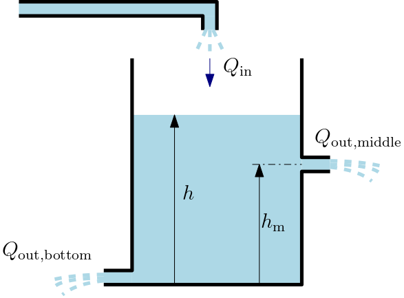
The model essentially expresses that the change in the volume is given by the difference between the inflow and the outflows. The outflows are proportional to the square root of the water level (Torricelli’s law) \dot V = \begin{cases} Q_\mathrm{in} - Q_\mathrm{out,middle} - Q_\mathrm{out,bottom}, & h>h_\mathrm{m}\\ Q_\mathrm{in} - Q_\mathrm{out,bottom}, & h\leq h_\mathrm{m} \end{cases}
Apparently things change when the water level crosses (in any direction) the height h_\mathrm{m}. This can be modelled using a hybrid automaton.

One lesson to learn from this example is that the transition from one mode to another is not necessarily due to some computer-controlled switch. Instead, it is our modelling choice. It is an approximation that assumes negligible diameter of the middle pipe. But taking into the consideration the volume of the tank, it is probably a justifiable approximation.
Example 4 (Bouncing ball) We assume that a ball is falling from some initial nonzero height above the table. After hitting the table, it bounces back, loosing a portion of the energy (the deformation is not perfectly elastic).
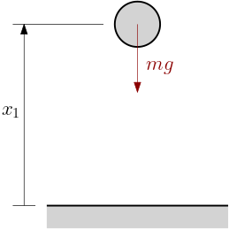
The state equation during the free fall is \dot{\bm x} = \begin{bmatrix} x_2\\ -g\end{bmatrix}, \quad \bm x = \begin{bmatrix}10\\0\end{bmatrix}.
But how can we model what happens during and after the collision? High-fidelity model would be complicated, involving partial differential equations to model the deformation of the ball and the table. These complexities can be avoided with a simpler model assuming that immediately after the collision the sign of the velocity abruptly (discontinuously) changes, and at the same time the ball also looses a portion of the energy.
When modelling this using a hybrid automaton, it turns out that we only need a single discrete state. The crucial feature of the model is then the nontrivial (non-identity) reset map. This is depicted in Fig. 6.

For completeness, here are the individual components of the hybrid automaton: \mathcal{Q} = \{q\}, \; \mathcal{Q}_0 = \{q\}
\mathcal{X} = \mathbb R^2, \; \mathcal{X}_0 = \left\{\begin{bmatrix}10\\0\end{bmatrix}\right\}
\mathcal{I} = \{\mathbb R^2 \mid x_1 > 0 \lor (x_1 = 0 \land x_2 \geq 0)\}
f(\bm x) = \begin{bmatrix} x_2\\ -g\end{bmatrix}
\mathcal{E} = \{(q,q)\}
\mathcal{G} = \{\bm x\in\mathbb R^2 \mid x_1=0 \land x_2 < 0\}
r((q,q),\bm x) = \begin{bmatrix}x_1\\ -\gamma x_2 \end{bmatrix}, where \gamma is the coefficient of restitution (e.g., \gamma = 0.9).
Some authors characterize the invariant set as x_1\geq 0. But this means that as the ball touches the ground, nothing forces it to leave the location and do the transition. Instead, the ball must penetrate the ground, however tiny distance, in order to trigger the transition. The current definition avoids this.
While the previous remark certainly holds, when solving the model numerically, the use of inequalities to define sets is inevitable. And some numerical solvers, in particular optimization solvers, cannot handle strict inequalities. That is perhaps why some authors are quite relaxed about this issue. We will encounter it later on.
Example 5 (Stick-slip friction model (Karnopp)) Consider a block of mass m placed freely on a surface. External horizontal force F_\mathrm{a} is applied to the block, setting it to a horizontaly sliding motion, against which the friction force F_\mathrm{f} is acting: m\dot v = F_\mathrm{a} - F_\mathrm{f}(v).
Common choice for a model of friction between two surfaces is Coulomb friction F_\mathrm{f}(v) = F_\mathrm{c}\operatorname*{sgn}(v).
The model is perfectly intuitive, isn’t it? Well, what if v=0 and F_\mathrm{a}<F_\mathrm{c}? Can you see the trouble?
One of the remedies is the Karnopp model of friction m\dot v = 0, \qquad v=0, \; |F_\mathrm{a}| < F_\mathrm{c} F_\mathrm{f} = \begin{cases}\operatorname*{sat}(F_\mathrm{a},F_\mathrm{c}), & v=0\\F_\mathrm{c}\operatorname*{sgn}(v), & \mathrm{else}\end{cases}
The model can be formulated as a hybrid automaton with two discrete states (modes, locations) as in Fig. 7.

Example 6 (Rimless wheel) A simple mechanical model that is occasionally used in the walking robot community is the rimless wheel rolling down a declined plane as depicted in Fig. 8.
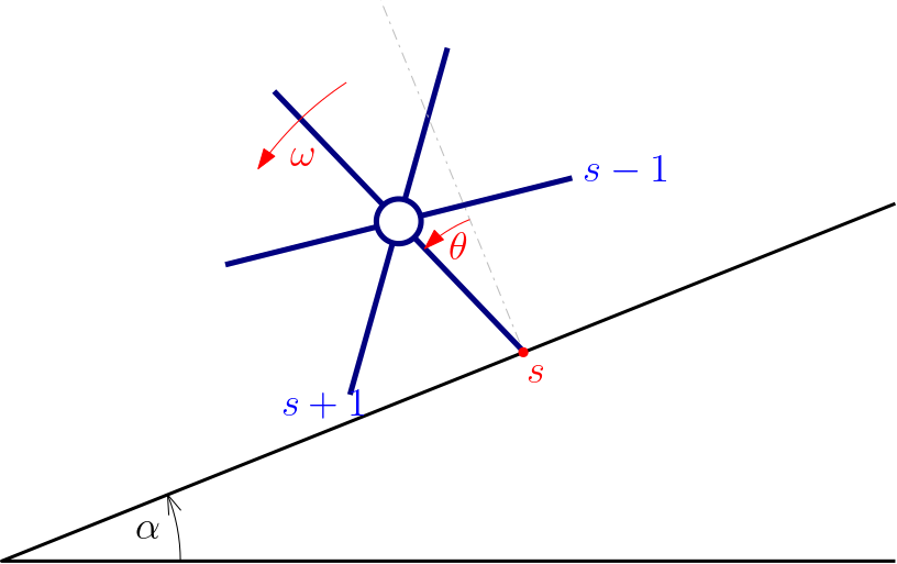
A hybrid automaton for the rimless wheel is below.

Alternatively, we do not represent the discrete state graphically as a node in the graph but rather as another – extending – state variable s \in \{0, 1, \ldots, 5\} within a single location.

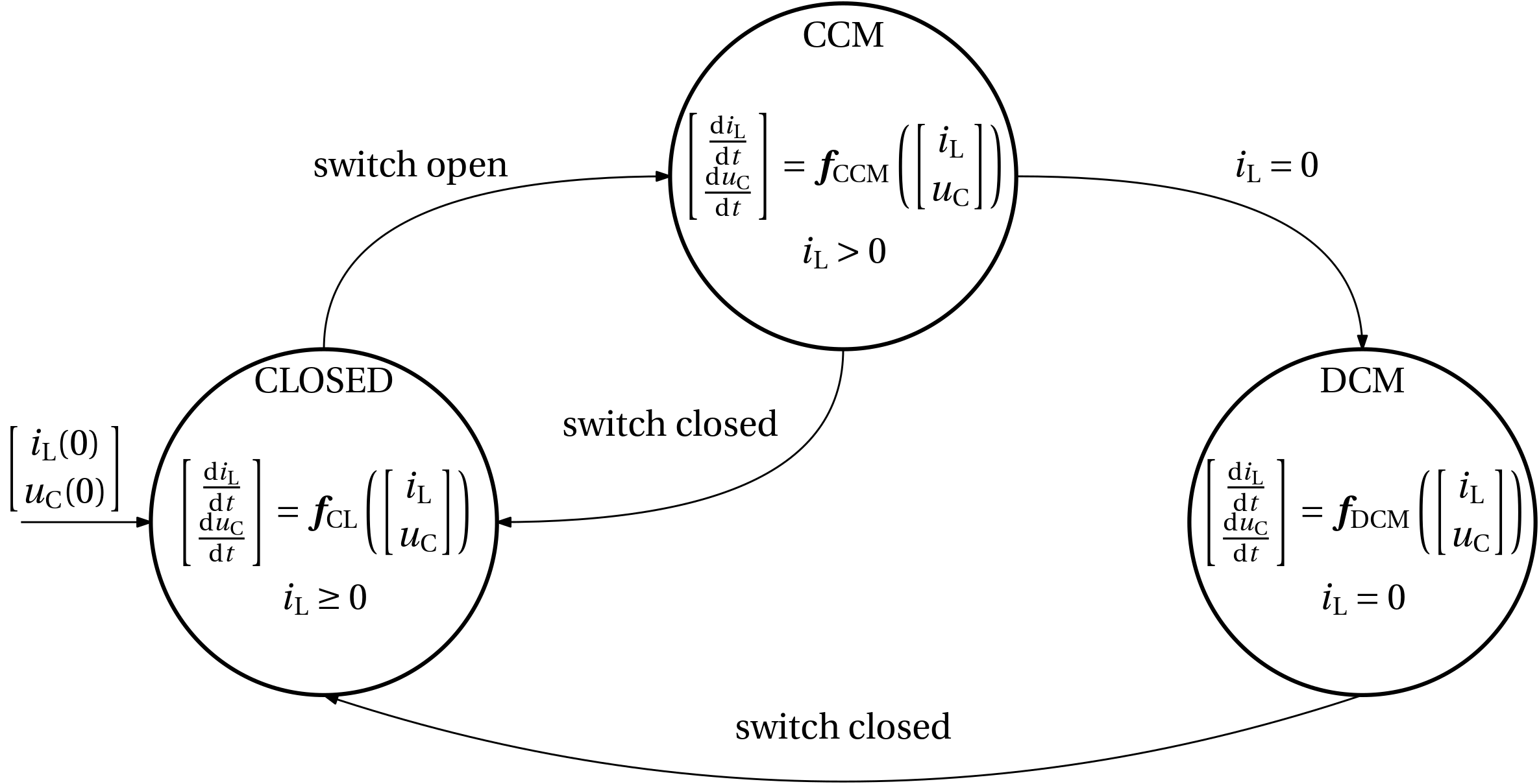
Example 7 (DC-DC boost converter) The enabling mechanism for a DC-DC converter is switching. Although the switching is realized with a semiconductor switch, for simplicity of the exposition we consider a manual switch in Fig. 11 below.
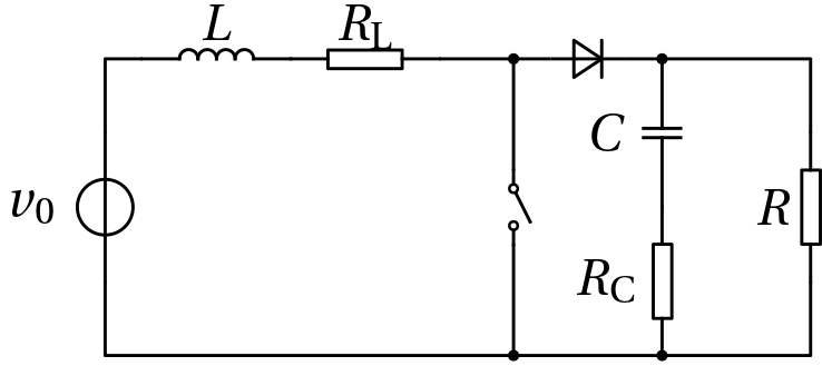
The switch introduces two modes of operation. But the (ideal) diode introduces a mode transition too.
The switch closed
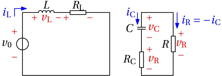
\begin{bmatrix} \frac{\mathrm{d}i_\mathrm{L}}{\mathrm{d}t}\\ \frac{\mathrm{d}v_\mathrm{C}}{\mathrm{d}t} \end{bmatrix} = \begin{bmatrix} -\frac{R_\mathrm{L}}{L}i_\mathrm{L} & 0\\ 0 & -\frac{1}{C(R+R_\mathrm{C})} \end{bmatrix} \begin{bmatrix} i_\mathrm{L}\\ v_\mathrm{C} \end{bmatrix} + \begin{bmatrix} \frac{1}{L}\\ 0 \end{bmatrix} v_0
Continuous conduction mode (CCM)
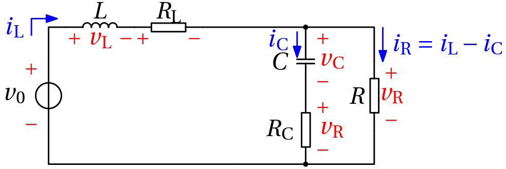
\begin{bmatrix} \frac{\mathrm{d}i_\mathrm{L}}{\mathrm{d}t}\\ \frac{\mathrm{d}v_\mathrm{C}}{\mathrm{d}t} \end{bmatrix} = \begin{bmatrix} -\frac{R_\mathrm{L}+ \frac{RR_\mathrm{C}}{R+R_\mathrm{C}}}{L} & -\frac{R}{L(R+R_\mathrm{C})}\\ \frac{R}{C(R+R_\mathrm{C})} & -\frac{1}{C(R+R_\mathrm{C})} \end{bmatrix} \begin{bmatrix} i_\mathrm{L}\\ v_\mathrm{C} \end{bmatrix} + \begin{bmatrix} \frac{1}{L}\\ 0 \end{bmatrix} v_0
Discontinuous cond. mode (DCM)
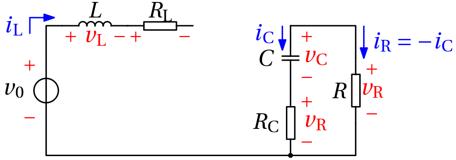
\begin{bmatrix} \frac{\mathrm{d}i_\mathrm{L}}{\mathrm{d}t}\\ \frac{\mathrm{d}v_\mathrm{C}}{\mathrm{d}t} \end{bmatrix} = \begin{bmatrix} 0 & 0\\ 0 & -\frac{1}{C(R+R_\mathrm{C})} \end{bmatrix} \begin{bmatrix} i_\mathrm{L}\\ v_\mathrm{C} \end{bmatrix} + \begin{bmatrix} 0\\ 0 \end{bmatrix} v_0
Possibly the events of opening and closing the switch can be driven by time: opening the switch is derived from the value of an input signal, closing the switch is periodic.
