Why complementarity constraints?
In this chapter we are going to present yet another framework for modelling hybrid systems, which comes with a rich theory and efficient algorithms. It is based on complementarity constraints. Before we introduce the modelling framework in the next section, we first explain the very concept of complementarity constraints and the related optimization problems.
Definition of complementarity constraints
Two variables x\in\mathbb R and y\in\mathbb R satisfy the complementarity constraint if x or y is equal to zero and both are nonnegative
xy=0, \; x\geq 0,\; y\geq 0,
or, using a dedicated compact notation
\boxed{0\leq x \perp y \geq 0.}
The or in the above definition is not exclusive, therefore it is possible that both x and y are zero.
The concept and notation extends to vectors x\in\mathbb R^n and y\in\mathbb R^n, in which case the constraint is interpreted componentwise \boxed{\bm 0\leq \bm x \perp \bm y \geq \bm 0.}
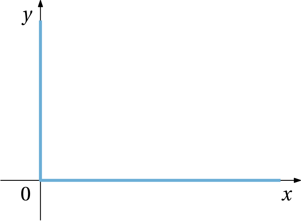
Geometric interpretation of complementarity constraints
The set of admissible pairs (x,y) in the \mathbb R^2 plane is constrained to the L-shaped subset given by the nonnegative x and y semi-axes (including the origin) as in Fig. 1.
Optimization over these constraints is difficult, and not only because the feasible set is nonconvex, but also because constraint qualification conditions are not satisfied. Still, some results and tools are available for some classes of optimization problems with these constraints.
Linear complementarity problem (LCP)
For a given square matrix \mathbf M and a vector \mathbf q , the linear complementarity problem (LCP) asks for finding two vectors \bm w and \bm z satisfying
\begin{aligned}
\bm w-\mathbf M\bm z &= \mathbf q, \\
\bm 0 \leq \bm w &\perp \bm z \geq \bm 0.
\end{aligned}
Just by moving all the provided data to the right-hand side we get \bm w = \underbrace{\mathbf M\bm z + \mathbf q}_{\mathbf f(\bm z)} and we can write the linear complementarity constraint compactly as \boxed{
\mathbf 0 \leq \mathbf M\bm z + \mathbf q \perp \bm z \geq \mathbf 0.}
\tag{1}
Existence of a unique solution
A unique solution exists for every vector \mathbf q if and only if the matrix \mathbf M is a P-matrix (something like positive definite, but not exactly, look it up yourself).
Nonlinear complementarity problem (NLCP)
Recall that when deriving Eq. 1, we denoted the right-hand side by \mathbf f(\bm x). The motivation for this was to help define a general nonlinear complementarity problem (NLCP): given a vector function \mathbf f: \mathbb R^n\rightarrow \mathbb R^n, find a vector \bm x\in\mathbb R^n satisfying \boxed{
\bm 0\leq \bm x \perp \mathbf f(\bm x) \geq \bm 0.}
\tag{2}
Mixed complementarity problem (MCP)
We now provide an extension of a complementarity constraint to the situation in which the variable x is lower- and upper-bounded. In particular, it can be stated as \boxed{
l \leq x \leq u \perp f(x),}
\tag{3}
where l and u are vectors of lower and upper bounds, respectively, and f(x) is a vector function which reads that
- if x is strictly within the interval, that is, l < x < u , then f(x)=0,
- if x= l , then f(x)\geq 0,
- if x= u , then f(x)\leq 0,
with elementwise interpretation in the vector case.
Extensions and related problems
LCP and MCP are all we need in our course, but let’s mentions some extensions and related problems.
Extended linear complementarity problem (ELCP)
Given some matrices \mathbf A and \mathbf B , vectors \mathbf c and \mathbf d , and m subsets \phi_j \sub \{1,2,\ldots,p\} , find a vector \bm x such that
\begin{aligned}
\sum_{j=1}^m\prod_{i\in\phi_j}(\mathbf A\bm x - \mathbf c)_i &= 0,\\
\mathbf A\bm x &\geq \mathbf c,\\
\mathbf B\bm x &= \mathbf d,
\end{aligned}
or show that no such \bm x exists.
The first equation is equivalent to
\forall j \in \{1, \ldots, m\} \; \exist i \in \phi_j \;\text{such that} \; (\mathbf A\bm x − \mathbf c)_i = 0.
Geometric interpretation: union of some faces of a polyhedron.
Mathematical program with complementarity constraints (MPCC)
The mathematical program with complementarity constraints (MPCC) is
\begin{aligned}
\operatorname*{minimize}_{\bm x\in\mathbb R^n} & \;f(\bm x)\\
\text{subject to} & \;\mathbf 0\leq \mathbf h(\bm x) \perp \mathbf g(\bm x) \geq \mathbf 0.
\end{aligned}
It is a special case of Mathematical program with equilibrium constraints (MPEC).
Mathematical program with equilibrium constraints (MPEC)
Optimization problem in which some variable should satisfy equilibrium constraints:
\begin{aligned}
\operatorname*{minimize}_{x_1,x_2} &\; f(x_1,x_2)\\
\text{subject to}&\; \nabla_{x_2} \phi(x_1,x_2) = 0.
\end{aligned}
For convex \phi() it can be reformulated into a Bilevel optimization problem.
Bilevel optimization
Optimization problem in which some variables are constrained to be results of some inner optimization. In the simplest form
\begin{aligned}
\operatorname*{minimize}_{x_1,x_2} &\; f(x_1,x_2)\\
\text{subject to}\ &\; x_2 = \text{arg}\,\min_{x_2} \;\phi(x_1,x_2).
\end{aligned}
Disjunctive constraints
Disjunctive constraints are given by a number of conditions induced by affine constraints and connected with \lor and \land logical operators
T_1 \lor T_2 \lor \ldots \lor T_m,
where
T_i = T_{i1} \land T_{i1} \land \ldots \land T_{in_{i}},
where
T_{ij} = \left[\mathbf c_{ij}\bm x + \mathbf d_{ij} \in \mathcal D_{ij}\right].
The connection of disjunctive constraints with complementarity constraints is straightforward:
\underbrace{(x\geq 0)}_{T_{11}} \land \underbrace{(xy = 0)}_{T_{12}} \land \underbrace{(y\geq 0)}_{T_{13}}.
Variational inequality (VI)
Given a set \mathcal K and a function F: \mathcal K \rightarrow \mathbb R^n, find a vector \bm x\in\mathcal K such that
\langle \mathbf F(\bm x), \bm y-\bm x \rangle \geq 0 \quad \forall \bm y\in\mathcal K.
If \mathbf F(\bm x) = \nabla f(\bm x) , VI is a convex optimization problem, that is, the problem of finding a vector \bm x\in\mathcal K such that
\langle \nabla f(\bm x), \bm y-\bm x \rangle \geq 0 \quad \forall \bm y\in\mathcal K.
But there may also be \mathbf F(\bm x) that is not the gradient of any function f(\bm x). In this regards, VI is a broader class of problems than convex optimization.
The reason why we include this problem class here is that if \mathcal K is a nonnegative orthant \mathbb R_{++}^n, that is, x_i \geq 0, \; i=1, \ldots, n , then the VI specializes to finding \bm x\geq \mathbf 0 such that
\langle \mathbf F(\bm x), \bm y-\bm x \rangle \geq 0 \quad \forall \bm y\geq \mathbf 0,
and it can be shown that it is equivalent to the NCP or LCP, depending on \mathbf F().
Proof. For \bm y=\bm 0, we get \langle \mathbf F(\bm x), -\bm x \rangle \geq 0, which is equivalent to \langle \mathbf F(\bm x), \bm x \rangle \leq 0. For \bm y = 2\bm x, we get \langle \mathbf F(\bm x), \bm x \rangle \geq 0. Reconciling the two inequalities, we get \langle \mathbf F(\bm x), \bm x \rangle = 0. Invoking the linearity of the inner product, we get \langle \mathbf F(\bm x), \bm y-\bm x \rangle = \langle \mathbf F(\bm x), \bm y\rangle \geq 0 \; \forall \bm y\geq \mathbf 0, from which it follows that \mathbf F(\bm x)\geq 0.
Similarly, if \mathcal K is a “box” in \mathbb R^n, that is, -\infty\leq l_i \leq x_i \leq u_i\leq \infty, \; i=1, \ldots, n, then VI is equivalent to the MCP. #TODO: sketch the explanation, if not a full proof.
Back to top